% thin space, limits underneath in displays % thin space, limits underneath in displays }}
Introduction and data used
We illustrate in this post the notion of ROC curves and Precision-Recall curves using both simple distributions (like Gaussian or uniform) but also data from a head-to-head benchmark evaluation of five SARS-CoV-2 serological assays (Ainsworth et al. 2020). We focus only on binary classification in this post.
For the empirical part, the underlying study compared the Abbott, DiaSorin, Oxford, Roche, and Siemens assays using a common set of well-characterized samples. We follow Ainsworth et al. (2020) and use a dataset that contains two groups of samples:
976 pre-pandemic samples, used as the known-negative reference group;
536 laboratory-confirmed SARS-CoV-2-positive samples, collected at least 20 days after symptom onset.
These groups contain a total of
\[
n = 976 + 536 = 1512
\]
observations. The proportion of positive samples in this dataset is therefore
An important distinction: this proportion describes the composition of the dataset, not necessarily the prevalence of SARS-CoV-2 infection in the population where a diagnostic test would be used. The sample composition may reflect how the study was designed and how samples were selected. This distinction will become important when interpreting precision–recall curves and average precision, which depend on the prevalence of positive cases.
The dataset (supplementary_dataset2.csv) is available here. The supplementary material of the associated paper describes the preprocessing used in this analysis.
Diagnostic testing: from one test to a family of tests
The message of this post
A diagnostic test is rarely a single test. It is a family\((\phi_t)_{t\in\mathbb{R}}\), indexed by a threshold \(t\).
ROC and precision/recall (PR) curves do not evaluate one test. They describe and compare the whole family at once, as \(t\) varies.
Setting: testing \(\mathcal{H}_0\) vs \(\mathcal{H}_1\)
Let \(Y\in\{0,1\}\) be the true health status:
\(\mathcal{H}_0\): “you are healthy” (\(Y=0\)),
\(\mathcal{H}_1\): “you are sick” (\(Y=1\)).
Health is presumed, like presumption of innocence in a courtroom. We reject \(\mathcal{H}_0\) (declare positive) only if the evidence is strong enough. The evidence is the measured value \(X\) (e.g., an antibody level). Write \[
\begin{align*}
X_0 & \sim \mathcal{L}(X\mid Y=0),\\
X_1 & \sim \mathcal{L}(X\mid Y=1),
\end{align*}
\] two independent variables. Conditioning on \(Y\) becomes an ordinary probability on \(X_0\) or \(X_1\).
A test, then a family of tests
A single test is a map \(\phi:\mathbb{R}\to[0,1]\). Here \(\phi(x)\) is the probability of declaring positive when \(X=x\).
\(\phi\in\{0,1\}\): hard decision,
\(\phi\in[0,1]\): randomized (soft) decision.
The prediction is then \(\hat Y\mid X \sim \mathrm{Bernoulli}(\phi(X))\).
Definition 1 (Family of tests) A family of tests is a collection \((\phi_t)_{t\in\mathbb{R}}\) of measurable maps \(\phi_t:\mathbb{R}\to[0,1]\). Here \(\phi_t(x)\) is the probability of declaring positive when \(X=x\) at threshold \(t\).
We assume that, for every \(x\in\mathbb{R}\):
(Monotone) for all \(t_1<t_2\), \[
\phi_{t_1}(x)\ge\phi_{t_2}(x),
\tag{1}\]
(Left-continuous) for all \(t\in\mathbb{R}\), \[
\phi_t(x)=\lim_{u\uparrow t}\phi_u(x),
\tag{2}\]
Note: \(\beta\) is the power of the test, not the Type II error, which is \(1-\beta\).
Theorem 1 (Score representation) The functions \(\alpha,\beta\) are non-increasing and left-continuous, with \[
\begin{align*}
\alpha(t+)&=\mathbb{E}[\phi_{t+}(X_0)],\\
\beta(t+)&=\mathbb{E}[\phi_{t+}(X_1)].
\end{align*}
\] Both tend to \(1\) at \(-\infty\) and to \(0\) at \(+\infty\).
Hence there exist independent real random variables \(T_0,T_1\) with \[
\begin{align*}
\mathbb{P}(T_0\ge t) & = \alpha(t),\\
\mathbb{P}(T_1\ge t) & = \beta(t).
\end{align*}
\tag{5}\]
▶Proof
By Equation 1, \(t\mapsto\phi_t(x)\) is non-increasing, so \(\alpha,\beta\) are non-increasing.
Since \(0\le\phi_t\le1\), dominated convergence with Equation 2, Equation 3 and the definition of \(\phi_{t+}\) gives: left-continuity of \(\alpha,\beta\), the identities for \(\alpha(t+),\beta(t+)\), and the limits \(1\) at \(-\infty\), \(0\) at \(+\infty\).
Hence \(F_0(t)\triangleq1-\alpha(t)\) is non-decreasing, left-continuous, with limits \(0\) and \(1\). It is the distribution function \(t\mapsto\mathbb{P}(T_0<t)\) of a unique law on \(\mathbb{R}\). Likewise for \(\beta\). Take \(T_0,T_1\) independent with these laws. In particular \[
\begin{align*}
\mathbb{P}(T_0>t)&=\alpha(t+),\\
\mathbb{P}(T_1>t)&=\beta(t+),\\
\mathbb{P}(T_0=t)&=\alpha(t)-\alpha(t+),\\
\mathbb{P}(T_1=t)&=\beta(t)-\beta(t+).
\end{align*}
\tag{6}\]
Any family of tests, however exotic, behaves like a plain threshold test on a hidden score:
healthy people have score \(T_0\),
sick people have score \(T_1\),
\(\phi_t\) “declares positive” when score \(\ge t\).
For \(\phi_t=\mathbb{1}\{g(x)\ge t\}\), simply \(T_j=g(X_j)\).
So we lose nothing by studying cut-offs \(T\ge t\). The ROC and PR curves below are built from \((\alpha(t),\beta(t))_{t}\).
Errors and the trade-off
Two errors are possible:
Type I (false positive): healthy person flagged, \[
\mathbb{P}(\text{Type I})
=\mathbb{P}(\hat Y_t=1\mid Y=0)=\alpha(t),
\]
Type II (false negative): sick person missed, \[
\mathbb{P}(\text{Type II})
=\mathbb{P}(\hat Y_t=0\mid Y=1)=1-\beta(t).
\]
Lowering \(t\) catches more sick people but flags more healthy ones. ROC and PR curves display this trade-off for all\(t\) simultaneously.
Naming and key quantities
The data are \(\{(Y_i,X_i)\}_{i=1,\dots,n}\), where \(Y_i\) is the true status of individual \(i\). Naming follows the classical terminology (see e.g., the Wikipedia article on ROC curves).
At a fixed \(t\), each sample falls in exactly one of four categories:
Note: the same color code is reused below. Red is for \(\mathrm{N}\), blue for \(\mathrm{P}\), crosses for a negative result, dots for a positive result.
The rates
Let \(\pi_1\triangleq\mathbb{P}(Y=1)\) and \(\pi_0\triangleq1-\pi_1\). We call \(\pi_1\) the prevalence.
Population rates (probabilities, not counts):
\(\mathrm{TPR}(t)=\mathbb{P}(\hat Y_t=1\mid Y=1)=\beta(t)\) (sensitivity, recall): sick people correctly detected,
\(\mathrm{FPR}(t)=\mathbb{P}(\hat Y_t=1\mid Y=0)=\alpha(t)\): healthy people wrongly flagged (the Type I error),
\(\mathrm{TNR}(t)=\mathbb{P}(\hat Y_t=0\mid Y=0)=1-\alpha(t)\) (specificity): healthy people correctly cleared,
\(\mathrm{Precision}(t)=\mathbb{P}(Y=1\mid\hat Y_t=1)\): people declared positive who are really sick.
By Equation 5, in terms of the scores: \[
\begin{align*}
\mathrm{TPR}(t)&=\mathbb{P}(T_1\ge t),\\
\mathrm{FPR}(t)&=\mathbb{P}(T_0\ge t),\\
\mathrm{TNR}(t)&=\mathbb{P}(T_0< t).
\end{align*}
\]
The first three depend only on the laws of \(X_0,X_1\). Precision also depends on \(\pi_0,\pi_1\) (exact form in Theorem 14 below). This is why PR curves react to prevalence and ROC curves do not.
Estimators. In practice \(t\), \(\pi_1\) and the laws of \(X_0,X_1\) are unknown. Each rate is estimated on a labeled sample by its empirical (plug-in) version: \[
\begin{align*}
\widehat{\mathrm{TPR}}(t) &=\frac{\mathrm{TP}(t)}{\mathrm{P}},\\
\widehat{\mathrm{TNR}}(t) &=\frac{\mathrm{TN}(t)}{\mathrm{N}},\\
\widehat{\mathrm{FPR}}(t) &=\frac{\mathrm{FP}(t)}{\mathrm{N}},\\
\widehat{\mathrm{Precision}}(t)
&=\frac{\mathrm{TP}(t)}{\hat{\mathrm{P}}_t}.
\end{align*}
\]
Sweeping \(t\) over \(\mathbb{R}\) turns these four numbers into curves. That is the next section.
The ROC curve
The receiver operating characteristic (ROC) curve comes from signal detection theory. This theory emerged from radar engineering during World War II and was formalised by Peterson, Birdsall, and Fox (1954).
The problem reads as follows: decide, from a noisy measurement, whether a target is present or only background noise. A receiver declares “signal” when the measurement exceeds a threshold. The ROC curve records how the detection rate and the false-alarm rate move together as the threshold varies.
This is the trade-off between catching true threats and raising false alarms. In the language of this post, it is the power of the family \((\phi_t)_t\) plotted against its Type I error.
In such a context, one test gives one point; a family of tests gives a curve.
Definition 2 (ROC curve) Let \((\phi_t)_{t\in\mathbb{R}}\) be a family of tests (Definition 1). For a threshold \(t\in\mathbb{R}\), the ROC operating point is the pair of false and true positive rates, \[
\begin{align*}
\mathrm{FPR}(t) & = \mathbb{E}[\phi_t(X_0)] = \alpha(t),\\
\mathrm{TPR}(t) & = \mathbb{E}[\phi_t(X_1)] = \beta(t).
\end{align*}
\]
The ROC curve is the curve traced by the operating point as \(t\) varies over \(\mathbb{R}\): \[
\{(\mathrm{FPR}(t), \mathrm{TPR}(t)) : t \in \mathbb{R}\}.
\]
For instance, for hard tests, \(\phi_t=\mathbb{1}\{X\ge t\}\), this reads \(\mathrm{FPR}(t)=\mathbb{P}(X_0\ge t)\) and \(\mathrm{TPR}(t)=\mathbb{P}(X_1\ge t)\).
By Equation 5, in terms of the scores, \[
\begin{align*}
\mathrm{FPR}(t) & = \mathbb{P}(T_0\ge t),\\
\mathrm{TPR}(t) & = \mathbb{P}(T_1\ge t).
\end{align*}
\] So the ROC curve of any family is that of a plain threshold test on \((T_0,T_1)\).
Properties.
Since FPR and TPR are probabilities, the curve lies in the unit square \([0,1]^2\).
By Equation 3, it goes from \((0,0)\) (as \(t\to+\infty\), nobody is flagged) to \((1,1)\) (as \(t\to-\infty\), everybody is flagged).
By Equation 1, both coordinates are non-increasing in \(t\), so the curve is monotone.
If \(T_0,T_1\) have atoms, the set of points has jumps. Several conventions exist to fill them:
Straight segments: randomize between the two neighboring tests. Every point on the segment is achievable by a randomized test,
Steps: a staircase (vertical, then horizontal), which makes no randomization assumption,
No filling: keep the isolated points.
The choice changes the look of the curve, and the value of quantities computed from it (e.g., the area under it). See Figure 3 below for a comparison on finite samples.
Properties
ROC endpoints
We now treat the two extreme classifiers (that do not depend on a threshold):
These are the two corner points of any ROC curve. The following lemma makes this precise.
Lemma 1 (ROC endpoints) Let \((\phi_t)_{t\in\mathbb{R}}\) be a family of tests (Definition 1). Then the ROC curve has the limiting endpoints \[
\boxed{
\lim_{t\to+\infty}
\bigl(\mathrm{FPR}(t),\mathrm{TPR}(t)\bigr)
=(0,0)
}
\] and \[
\boxed{
\lim_{t\to-\infty}
\bigl(\mathrm{FPR}(t),\mathrm{TPR}(t)\bigr)
=(1,1).
}
\]
▶Proof
By definition, for \(j\in\{0,1\}\), \[
\begin{align*}
\mathrm{FPR}(t) &= \mathbb{E}[\phi_t(X_0)] = \alpha(t),\\
\mathrm{TPR}(t) &= \mathbb{E}[\phi_t(X_1)] = \beta(t).
\end{align*}
\]
Step 1: limit as \(t\to+\infty\). By Equation 3, \(\phi_t(X_j)\to0\) pointwise. Since \(0\le\phi_t(X_j)\le1\), dominated convergence gives \[
\mathbb{E}[\phi_t(X_j)]\to0,
\] hence \[
\boxed{\lim_{t\to+\infty} \bigl(\mathrm{FPR}(t),\mathrm{TPR}(t)\bigr) = (0,0).}
\]
Step 2: limit as \(t\to-\infty\). By Equation 3, \(\phi_t(X_j)\to1\) pointwise. Dominated convergence again gives \[
\mathbb{E}[\phi_t(X_j)]\to1,
\] hence \[
\boxed{\lim_{t\to-\infty} \bigl(\mathrm{FPR}(t),\mathrm{TPR}(t)\bigr) = (1,1).}
\]
The point \((0,0)\) corresponds to a classifier that never declares a signal (no false‑positives, no true‑positives); the point \((1,1)\) corresponds to a classifier that always declares a signal (maximal false‑positives and maximal true‑positives).
Every ROC curve for a finite scoring rule must start at \((0,0)\) and end at \((1,1)\); the two extreme tests are precisely these endpoints, as formalized below:
Extreme cases
ROC curve for a perfect classifier
Theorem 2 (ROC curve for a perfect classifier) Suppose there exists a threshold \(t^\star \in \mathbb{R}\) such that \[
\mathbb{E}(\phi_{t^\star}(X_0)) = 0, \quad \mathbb{E}(\phi_{t^\star}(X_1)) = 1.
\] Then, \[
\boxed{\mathrm{FPR}(t^\star) = 0, \quad \mathrm{TPR}(t^\star) = 1,}
\] and the ROC curve passes through the upper-left corner \((0,1)\) for \(t^\star\).
▶Proof
By definition, \(\mathrm{FPR}(t^\star) = \mathbb{E}(\phi_{t^\star}(X_0))) = 0\) and \(\mathrm{TPR}(t^\star) = \mathbb{E}(\phi_{t^\star}(X_1)) = 1\). Thus the threshold \(t^\star\) yields the operating point \((0,1)\), representing perfect discrimination.
ROC curve for an always-wrong classifier
Corollary 1 (ROC curve for an always-wrong classifier) Suppose there exists a threshold \(t^\star \in \mathbb{R}\) such that \[
\mathbb{E}(\phi_{t^\star}(X_0)) = 1, \quad \mathbb{E}(\phi_{t^\star}(X_1)) = 0.
\] Then, \[
\boxed{\mathrm{FPR}(t^\star) = 1, \quad \mathrm{TPR}(t^\star) = 0,}
\] and the ROC curve passes through the lower-right corner \((1,0)\).
▶Proof
By definition, \(\mathrm{FPR}(t^\star) = \mathbb{E}(\phi_{t^\star}(X_0)) = 1\) and \(\mathrm{TPR}(t^\star) = \mathbb{E}(\phi_{t^\star}(X_1)) = 0\). Thus the threshold \(t^\star\) yields the operating point \((1,0)\), representing perfectly inverted discrimination.
ROC curve under random guessing
Theorem 3 (ROC curve under random guessing) Suppose \(X_0 \stackrel{d}{=} X_1\). Then, for every \(t \in \mathbb{R}\), \[
\boxed{\mathrm{FPR}(t) = \mathrm{TPR}(t).}
\] Consequently, the ROC curve lies on the diagonal line \(u=v\) of the unit square.
▶Proof
Since \(X_0 \stackrel{d}{=} X_1\), \(\mathbb{P}(\phi_t(X_0) = 1) = \mathbb{E}(\phi_t(X_1))\) for every \(t \in \mathbb{R}\), so \(\mathrm{FPR}(t) = \mathrm{TPR}(t)\) for all \(t\), and the ROC curve is included in the diagonal line.
Monotonicity of ROC curves
Monotonicity is built into the definition of a family of tests (Definition 1). It is the nested condition Equation 1: for all \(x\in\mathbb{R}\), \[
t_1<t_2\;\implies\;\phi_{t_1}(x)\ge\phi_{t_2}(x).
\]
It transfers to the ROC coordinates. It covers hard cut-offs \(\mathbb{1}\{x\ge t\}\), scores \(\mathbb{1}\{g(x)\ge t\}\) and sigmoids \(\sigma(g(x)-t)\).
Theorem 4 (Monotonicity of ROC curves) Let \((\phi_t)_{t\in\mathbb{R}}\) be a family of tests (Definition 1). Then for all \(t_1<t_2\), \[
\begin{align*}
\mathrm{TPR}(t_1)&\ge\mathrm{TPR}(t_2),\\
\mathrm{FPR}(t_1)&\ge\mathrm{FPR}(t_2).
\end{align*}
\]
In words: both rates are non-increasing as the threshold increases.
▶Proof
Recall that \[
\begin{align*}
\mathrm{TPR}(t)&=\mathbb{E}[\phi_t(X_1)]=\beta(t),\\
\mathrm{FPR}(t)&=\mathbb{E}[\phi_t(X_0)]=\alpha(t).
\end{align*}
\]
Fix \(t_1<t_2\). By Equation 1, pointwise in \(x\), \[
\phi_{t_1}(x)\ge\phi_{t_2}(x).
\] Hence, for every outcome \(\omega\) and for \(j\in\{0,1\}\), \[
\phi_{t_1}(X_j(\omega))\ge\phi_{t_2}(X_j(\omega)).
\]
Both variables are bounded in \([0,1]\), so their expectations exist. Expectation preserves order, so \[
\mathbb{E}[\phi_{t_1}(X_j)]
\ge
\mathbb{E}[\phi_{t_2}(X_j)],
\qquad j\in\{0,1\}.
\]
Invariance of ROC curves under increasing transforms
Let \(g:\mathbb{R}\to\mathbb{R}\) be a strictly increasing bijection, and set \(Z_j=g(X_j)\), \(j\in\{0,1\}\) and \(Z=g(X)\).
We relabel the family to act on the transformed data: \[
\widetilde\phi_t(z)
\triangleq
\phi_{g^{-1}(t)}\bigl(g^{-1}(z)\bigr),
\qquad t,z\in\mathbb{R}.
\tag{7}\]
Its rates on \(Z\) are \[
\begin{align*}
\mathrm{FPR}_{Z}(t)
&=\mathbb{E}[\widetilde\phi_t(Z_0)],\\
\mathrm{TPR}_{Z}(t)
&=\mathbb{E}[\widetilde\phi_t(Z_1)].
\end{align*}
\]
Theorem 5 (Invariance under strictly increasing transforms) Let \((\phi_t)_{t\in\mathbb{R}}\) be a family of tests (Definition 1), and \(g\) a strictly increasing bijection. Then:
\((\widetilde\phi_t)_{t\in\mathbb{R}}\) is a family of tests (Definition 1),
for every \(t\in\mathbb{R}\), \[
\boxed{
\begin{aligned}
\mathrm{FPR}_{Z}(t)&=\mathrm{FPR}_X\bigl(g^{-1}(t)\bigr),\\
\mathrm{TPR}_{Z}(t)&=\mathrm{TPR}_X\bigl(g^{-1}(t)\bigr).
\end{aligned}}
\]
the two ROC curves coincide: \[
\{(\mathrm{FPR}_{Z}(t),\mathrm{TPR}_{Z}(t)):t\in\mathbb{R}\}
=
\{(\mathrm{FPR}_X(s),\mathrm{TPR}_X(s)):s\in\mathbb{R}\}.
\]
Only the labelling of the points by a threshold changes, through the increasing map \(t\mapsto g^{-1}(t)\).
▶Proof
Step 1: \(\widetilde\phi\) is a family of tests. The map \(g^{-1}\) is a strictly increasing bijection of \(\mathbb{R}\), hence continuous, with \(g^{-1}(t)\to\pm\infty\) as \(t\to\pm\infty\). Fix \(z\in\mathbb{R}\) and set \(x=g^{-1}(z)\).
Nested. If \(t_1<t_2\), then \(g^{-1}(t_1)<g^{-1}(t_2)\). By Equation 1, \(\widetilde\phi_{t_1}(z)\ge\widetilde\phi_{t_2}(z)\).
Left-continuous. If \(u\uparrow t\), then \(g^{-1}(u)\uparrow g^{-1}(t)\) strictly from below. By Equation 2, \(\widetilde\phi_u(z)\to\widetilde\phi_t(z)\).
Boundary. By Equation 3 and the limits of \(g^{-1}\), \(\widetilde\phi_t(z)\to1\) as \(t\to-\infty\) and \(\to0\) as \(t\to+\infty\).
Step 2: pointwise identity. Take \(z=g(x)\). Then \(g^{-1}(z)=x\), so \[
\widetilde\phi_t\bigl(g(x)\bigr)
=\phi_{g^{-1}(t)}(x).
\tag{8}\]
Step 3: rates. Since \(Z_j=g(X_j)\), Equation 8 gives \(\widetilde\phi_t(Z_j)=\phi_{g^{-1}(t)}(X_j)\) as random variables. Taking expectations, \[
\begin{align*}
\mathrm{FPR}_{g(X)}(t)
&=\mathbb{E}[\phi_{g^{-1}(t)}(X_0)]
=\mathrm{FPR}_X\bigl(g^{-1}(t)\bigr),\\
\mathrm{TPR}_{g(X)}(t)
&=\mathbb{E}[\phi_{g^{-1}(t)}(X_1)]
=\mathrm{TPR}_X\bigl(g^{-1}(t)\bigr).
\end{align*}
\]
Step 4: curves. Since \(g^{-1}\) is a bijection of \(\mathbb{R}\), \(s=g^{-1}(t)\) runs over all of \(\mathbb{R}\) as \(t\) does. So both sets of points are the same.
Special cases and scores.
For \(\phi_t(x)=\mathbb{1}\{x\ge t\}\), \[
\widetilde\phi_t(z)
=\mathbb{1}\{g^{-1}(z)\ge g^{-1}(t)\}
=\mathbb{1}\{z\ge t\}.
\] So the cut-off on \(Z=g(X)\) has the same ROC curve as the cut-off on \(X\).
In terms of Theorem 1, the score of \(\widetilde\phi\) is \(g(T_j)\): \(\mathbb{P}(g(T_j)\ge t)
=\mathbb{P}(T_j\ge g^{-1}(t))\).
Only the ranking of scores matters, not their scale.
Symmetries of ROC curves
Reversing the decision rule and/or swapping the class labels acts on the ROC curve as an exact affine reflection of the unit square.
Write \(\mathcal{C}\) for the ROC curve of a family \((\phi_t)_t\) (Definition 2). Consider the three maps of the square: \[
\begin{align*}
R(x,y)&=(1-x,\,1-y),\\
S(x,y)&=(y,\,x),\\
R\circ S\,(x,y)&=(1-y,\,1-x).
\end{align*}
\]
They are the central reflection about \((\tfrac12,\tfrac12)\), the reflection about \(y=x\), and the reflection about \(y=1-x\).
Why prevalence plays no role.\(\mathrm{FPR}\) and \(\mathrm{TPR}\) depend only on the laws of \(X_0\) and \(X_1\), never on \(\pi_0,\pi_1\). So all three symmetries are statements about these two laws.
Test reversal
Keep the labels, reverse the rule. Raising the threshold must still make the test less positive, so we reindex and use right limits: \[
\phi^{\mathrm{rev}}_t(x)
\triangleq
1-\phi_{(-t)+}(x),
\qquad t\in\mathbb{R}.
\tag{9}\]
The operating point is sent to \[
\boxed{
\binom{\mathrm{FPR}(t)}{\mathrm{TPR}(t)}
\longmapsto
\binom{1-\mathrm{FPR}(t)}{1-\mathrm{TPR}(t)}
}
\] (exactly so when \(\alpha,\beta\) are continuous; otherwise see the proof).
Theorem 6 (Central symmetry) Let \((\phi_t)_{t\in\mathbb{R}}\) be a family of tests (Definition 1). Then:
\((\phi^{\mathrm{rev}}_t)_{t\in\mathbb{R}}\) is a family of tests,
its ROC curve is \(R(\mathcal{C})\), the central reflection of \(\mathcal{C}\) about \((\tfrac12,\tfrac12)\).
▶Proof
Step 1: a family of tests. Fix \(x\) and put \(s=-t\).
Nested. If \(t_1<t_2\), then \(-t_1>-t_2\). By Equation 1, \(\phi_{(-t_1)+}(x)\le\phi_{(-t_2)+}(x)\), so \(\phi^{\mathrm{rev}}_{t_1}(x)\ge\phi^{\mathrm{rev}}_{t_2}(x)\).
Left-continuous. If \(u\uparrow t\), then \(-u\downarrow -t\), so \(\phi_{(-u)+}(x)\to\phi_{(-t)+}(x)\).
Boundary. As \(t\to-\infty\), \(-t\to+\infty\) and \(\phi_{(-t)+}(x)\to0\), so \(\phi^{\mathrm{rev}}_t(x)\to1\). Symmetrically, \(\phi^{\mathrm{rev}}_t(x)\to0\) as \(t\to+\infty\).
Step 2: rates. By Theorem 1, \(\mathbb{E}[\phi_{s+}(X_j)]=\alpha(s+)\) or \(\beta(s+)\). Hence \[
\begin{align*}
\mathrm{FPR}^{\mathrm{rev}}(t)
&=1-\alpha\bigl((-t)+\bigr),\\
\mathrm{TPR}^{\mathrm{rev}}(t)
&=1-\beta\bigl((-t)+\bigr).
\end{align*}
\]
Step 3: curve. With \(s=-t\), the operating points are \(R\bigl(\alpha(s+),\beta(s+)\bigr)\), \(s\in\mathbb{R}\). These are the right-limit points of \(\mathcal{C}\). At a jump, they are the endpoints of the filled segment, and \(R\) maps segments to segments. Hence the ROC curve of the reversed family is \(R(\mathcal{C})\). If \(\alpha,\beta\) are continuous, \(\alpha(s+)=\alpha(s)\) and this is just \((\mathrm{FPR},\mathrm{TPR})\mapsto(1-\mathrm{FPR},1-\mathrm{TPR})\).
Class label swap
Keep the rule, swap the labels: \(Y'=1-Y\), so \(X_0'=X_1\) and \(X_1'=X_0\). The operating point is sent to \[
\boxed{
\binom{\mathrm{FPR}(t)}{\mathrm{TPR}(t)}
\longmapsto
\binom{\mathrm{TPR}(t)}{\mathrm{FPR}(t)}.
}
\]
Theorem 7 (Main-diagonal symmetry) Let \((\phi_t)_{t\in\mathbb{R}}\) be a family of tests (Definition 1). With the labels swapped and the family unchanged, the ROC curve is \(S(\mathcal{C})\), the reflection of \(\mathcal{C}\) about the diagonal \(y=x\).
▶Proof
The family is unchanged, so it is still a family of tests. Only the roles of \(X_0,X_1\) are exchanged: \[
\begin{align*}
\mathrm{FPR}'(t)&=\mathbb{E}[\phi_t(X_0')]
=\mathbb{E}[\phi_t(X_1)]=\mathrm{TPR}(t),\\
\mathrm{TPR}'(t)&=\mathbb{E}[\phi_t(X_1')]
=\mathbb{E}[\phi_t(X_0)]=\mathrm{FPR}(t).
\end{align*}
\] So \((\mathrm{FPR}',\mathrm{TPR}')(t)=S(\mathrm{FPR},\mathrm{TPR})(t)\) for every \(t\). \(S\) is affine, so it also maps filled segments to filled segments.
Label swap with test reversal
Swap the labels and reverse the rule (Equation 9). The operating point is sent to \[
\boxed{
\binom{\mathrm{FPR}(t)}{\mathrm{TPR}(t)}
\longmapsto
\binom{1-\mathrm{TPR}(t)}{1-\mathrm{FPR}(t)}.
}
\]
Theorem 8 (Anti-diagonal symmetry) Let \((\phi_t)_{t\in\mathbb{R}}\) be a family of tests (Definition 1). With the labels swapped and the rule reversed, the ROC curve is \((R\circ S)(\mathcal{C})\), the reflection of \(\mathcal{C}\) about the anti-diagonal \(y=1-x\).
▶Proof
Apply Theorem 6 to the family \((\phi_t)\), then Theorem 7 to the reversed family (a family of tests by Step 1). The two reflections compose to \[
R\circ S\,(x,y)=(1-y,\,1-x).
\] Concretely, with \(s=-t\), \(\mathrm{FPR}'(t)=1-\beta(s+)\) and \(\mathrm{TPR}'(t)=1-\alpha(s+)\). Since \(R\circ S=S\circ R\), the order of the two operations does not matter.
Consequences.
Reversing a worse-than-chance test makes it better than chance (reflection about \((\tfrac12,\tfrac12)\)).
A curve symmetric under \(S\) is unchanged by label swapping.
The curve of any “worse than chance” family can be improved by reversing it.
Summary and visualization
Table 1: Transformations of the ROC operating point. Reversal: \(X<t \leftrightarrow X\ge t\); label swap: \(Y=0\leftrightarrow Y=1\).
Transformation
FPR\('\) / TPR\('\)
Geometry
Test reversal
\(1-\mathrm{FPR}\) / \(1-\mathrm{TPR}\)
Central symmetry, center \((0.5,0.5)\)
Label swap
\(\mathrm{TPR}\) / \(\mathrm{FPR}\)
Main diagonal \(y=x\)
Reversal + swap
\(1-\mathrm{TPR}\) / \(1-\mathrm{FPR}\)
Anti-diagonal \(y=1-x\)
These three transformations creat reflected copy shape. As noted above, none of them depends on the class prevalence \(\pi_1\). You can verify this directly with the interactive below.
Interactive ROC curve exploration. The visualization below illustrates these properties for a Gaussian model \(X\mid Y=0\sim\mathcal N(0,1)\), \(X\mid Y=1\sim\mathcal N(1,2^2)\). Use the Threshold slider to move along the ROC curve and watch the operating point change; the Prevalence (\(\pi_1\)) slider confirms that the ROC curve itself is unaffected by class imbalance, however that slider is moved. The plot also shows the reversed-rule and class-inverted curves described above.
Figure 1: ROC curve under symmetry transformations
ROC curves for common distributions
Below we summarize the ROC curves for classic location-scale distributions, along with the exponential case. Throughout, we assume that \(Z_0, Z_1\) are independent and identically distributed with a common continuous CDF \(F\). The tests considered here are written as \(\mathbb{1}(X \ge t)\). We define the location-scale variables as:
\[
\begin{align*}
X_0 & = \sigma_0 Z_0 + \mu_0,\\
X_1 & = \sigma_1 Z_1 + \mu_1,
\end{align*}
\] where \(\sigma_0 > 0\) and \(\sigma_1 > 0\) are the scale parameters, and \(\mu_0, \mu_1 \in \mathbb{R}\) are the location parameters. We use the following notation:
Where the table comes from. All the rows follow from a single identity (Theorem 22): for \(X_y=\sigma_yZ_y+\mu_y\) with \(Z_0,Z_1\) i.i.d. with CDF \(F\), \[
\mathrm{TPR}\!=\!1\!-\!F\bigl(\rho\,F^{-1}(1\!-\!\mathrm{FPR})\!-\!\Delta\bigr),
\] which simplifies to \(\mathrm{TPR}=F\bigl(\Delta+\rho\,F^{-1}(\mathrm{FPR})\bigr)\) when \(F\) is symmetric (Corollary 3). The statements, the proofs, and the row-by-row computations (Gaussian, Cauchy, Logistic, Uniform, Gumbel, Exponential) are collected in Appendix A.
Visualization
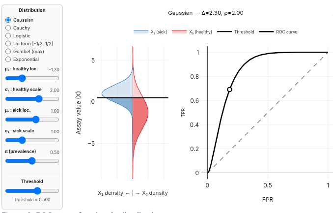
The widget below lets you explore Theorem 22 interactively for the distribution described in Table 2. Use the sliders on the left to set \(\mu_0,\sigma_0\) (healthy class) and \(\mu_1,\sigma_1\) (sick class), and drag the Threshold slider to move \(t\).
The middle panel shows the two population densities plotted vertically: \(X_1\) (sick) on the left in blue, \(X_0\) (healthy) on the right in red. The horizontal black line marks the current threshold \(t\); the darker-shaded region of each density is \(\{X<t\}\) (the portion of that class predicted negative under the rule \(\hat{Y}_t=\mathbb{1}\{X\ge t\}\)) while the lighter region above the line is predicted positive.
The right panel shows the theoretical ROC curve for the current \((\mu_0,\sigma_0,\mu_1,\sigma_1)\), with the dashed diagonal as the random-guessing reference (Theorem 3) and a marker at the operating point \((\mathrm{FPR}(t),\mathrm{TPR}(t))\) corresponding to the threshold you’ve selected, so you can see exactly which point on the curve a given threshold produces, and watch the curve itself deform as you change the means, standard deviations, or their ratio \(\rho=\tfrac{\sigma_0}{\sigma_1}\).
The title above the plot reports the current \(\Delta=\tfrac{(\mu_1-\mu_0)}{\sigma_1}\), \(\rho = \tfrac{\sigma_0}{\sigma_1}\).
Figure 2: ROC curve for classic distributions
Note: Visually, the TPR is the ratio of the light blue area over the full blue area on the left, while the FPR is the ratio of the light red area over the full red area (right).
Interpretation
\(\Delta=(\mu_1-\mu_0)/\sigma_1\) measures the (scale-standardized) separation between \(X_0\) and \(X_1\); \(\rho=\sigma_0/\sigma_1\) compares their spread. Together they set the difficulty and shape of the ROC curve.
\(\rho=1\): the usual equal-scale model, \(\mathrm{TPR}=F(\Delta+F^{-1}(\mathrm{FPR}))\) for symmetric \(F\), e.g., the binormal case \(\mathrm{TPR}=\Phi(\Delta+\Phi^{-1}(\mathrm{FPR}))\).
\(\Delta=0,\ \rho=1\):\(X_0\stackrel{d}{=}X_1\), and the ROC curve is the diagonal (random guessing). Note \(\Delta=0\) alone is not enough when \(\rho\ne1\): equal location with unequal scale still separates the classes, via spread rather than location.
\(\rho\ne1\): the curve need not be symmetric about the anti-diagonal or concave everywhere, if \(\rho<1\) (sick population more dispersed), the curve can dip toward the diagonal near one corner before rising, a non-concave S-shape sometimes seen in real assay data.
\(\Delta\to\infty\) (fixed \(\rho\)): the classes separate perfectly, and the curve approaches the ideal curve through \((0,1)\).
Now we illustrate the empirical counterpart, when one samples elements from the distributions but without access to the true densities.
Figure 3: Empirical counterpart of ROC curve for classic distributions.
ROC curves are commonly displayed with stepwise (vertical and horizontal) segments, but using affine interpolation between points provides a more informative visualization. In particular, the affine approach better reveals non-concavities in the curve, offering clearer insights into classifier performance and highlighting suboptimal decision thresholds (as explained below). Smooth interpolation distinguishes subtle variations in behavior that would otherwise be obscured by the sharp transitions of stepwise plots.
ROC curves and Neyman-Pearson
So far, a family \((\phi_t)_t\) gave one ROC curve. Now we ask the converse question: how good can a ROC curve be? We need two tools: randomization, and the likelihood ratio.
Randomized mixtures
Let \(\mathcal{T}\) be the set of all measurable tests \(\phi:\mathbb{R}\to[0,1]\). For \(\phi\in\mathcal{T}\), write \[
\begin{align*}
\mathrm{FPR}(\phi)&=\mathbb{E}[\phi(X_0)],\\
\mathrm{TPR}(\phi)&=\mathbb{E}[\phi(X_1)].
\end{align*}
\] This extends the rates of \(\phi_t\) to any single test.
Theorem 9 (Randomized mixtures) Let \(\phi,\phi'\in\mathcal{T}\) with operating points \(P=(\mathrm{FPR}(\phi),\mathrm{TPR}(\phi))\) and \(P'=(\mathrm{FPR}(\phi'),\mathrm{TPR}(\phi'))\). For \(\lambda\in[0,1]\), set \[
\phi_\lambda\triangleq\lambda\phi+(1-\lambda)\phi'.
\] Then \(\phi_\lambda\in\mathcal{T}\), and \[
\begin{align*}
\mathrm{FPR}(\phi_\lambda)&=\lambda\,\mathrm{FPR}(\phi)+(1-\lambda)\,\mathrm{FPR}(\phi'),\\
\mathrm{TPR}(\phi_\lambda)&=\lambda\,\mathrm{TPR}(\phi)+(1-\lambda)\,\mathrm{TPR}(\phi').
\end{align*}
\] As \(\lambda\) goes from \(0\) to \(1\), the operating point sweeps the segment \([P,P']\).
▶Proof
\(\phi_\lambda\) is measurable with values in \([0,1]\), as a convex combination of such maps. Linearity of expectation gives both identities. The map \(\lambda\mapsto\lambda P+(1-\lambda)P'\) parametrizes \([P,P']\).
Interpretation.\(\phi_\lambda(x)\) is the probability of declaring positive when we flip a coin: use \(\phi\) with probability \(\lambda\), \(\phi'\) otherwise. This justifies the straight-segment convention for filling jumps of a ROC curve: two neighboring tests of a family can always be mixed.
Let \(\mathcal{R}\triangleq\{(\mathrm{FPR}(\phi),\mathrm{TPR}(\phi)):\phi\in\mathcal{T}\}\) be the attainable region.
It contains \((0,0)\) and \((1,1)\) (take \(\phi\equiv0\) and \(\phi\equiv1\)).
It is symmetric under \(R\), the central symmetry of center \((1/2, 1/2)\) (take \(1-\phi\)): \(R(\mathcal{R})=\mathcal{R}\).
Hence only the upper boundary of \(\mathcal{R}\) matters. Any point below it is matched or beaten by mixing two tests on the boundary. The next theorem identifies this boundary.
The likelihood-ratio test
Assume \(X_0,X_1\) have densities \(f_0,f_1\) with respect to a common \(\sigma\)-finite measure \(\mu\), and \(f_0>0\)\(\mu\)-a.e. Define the likelihood ratio\[
L(x)\triangleq\frac{f_1(x)}{f_0(x)}\in[0,\infty).
\]
For \(k\in[0,\infty]\) and \(\gamma\in[0,1]\), set \[
\phi^{\mathrm{LR}}_{k,\gamma}(x)=
\begin{cases}
1 & L(x)>k,\\
\gamma & L(x)=k,\\
0 & L(x)<k.
\end{cases}
\]
Lemma 2 (Exact level) For every \(\alpha\in[0,1]\) there exist \(k_\alpha\in[0,\infty]\) and \(\gamma_\alpha\in[0,1]\) such that \[
\mathrm{FPR}\bigl(\phi^{\mathrm{LR}}_{k_\alpha,\gamma_\alpha}\bigr)=\alpha.
\] We write \(\phi^{\mathrm{LR}}_\alpha\triangleq\phi^{\mathrm{LR}}_{k_\alpha,\gamma_\alpha}\).
▶Proof
Let \(H(k)\triangleq\mathbb{P}(L(X_0)>k)\). It is non-increasing and right-continuous, with \(H(\infty)=0\) and \(H(0)\le1\). Set \(k_\alpha\triangleq\inf\{k\ge0:H(k)\le\alpha\}\).
If \(k_\alpha=\infty\), then \(\alpha=0\) and \(\phi^{\mathrm{LR}}_\alpha\equiv0\) (\(\mu\)-a.e., since \(f_0>0\)).
Otherwise, right-continuity gives \(H(k_\alpha)\le\alpha\le H(k_\alpha-)\), and \(H(k_\alpha-)-H(k_\alpha)=\mathbb{P}(L(X_0)=k_\alpha)\). If this probability is \(0\), take \(\gamma_\alpha=0\). If not, take \[
\gamma_\alpha=\frac{\alpha-H(k_\alpha)}{\mathbb{P}(L(X_0)=k_\alpha)}\in[0,1].
\]
In both cases, \(\mathbb{E}[\phi^{\mathrm{LR}}_\alpha(X_0)] =H(k_\alpha)+\gamma_\alpha\,\mathbb{P}(L(X_0)=k_\alpha)=\alpha\).
Theorem 10 (Neyman–Pearson optimality) For every \(\alpha\in[0,1]\), \(\phi^{\mathrm{LR}}_\alpha\) has the highest true positive rate among all tests of level \(\alpha\): \[
\boxed{
\mathrm{TPR}(\phi^{\mathrm{LR}}_\alpha)
=\sup\bigl\{\mathrm{TPR}(\phi):\phi\in\mathcal{T},\ \mathrm{FPR}(\phi)=\alpha\bigr\}.
}
\] Set \(\beta^\star(\alpha)\triangleq\mathrm{TPR}(\phi^{\mathrm{LR}}_\alpha)\). Then:
the point \((\alpha,\beta^\star(\alpha))\) lies on or above every operating point \((\mathrm{FPR}(\phi),\mathrm{TPR}(\phi))\), \(\phi\in\mathcal{T}\) (upper envelope),
\(\beta^\star\) is concave on \([0,1]\).
▶Proof
Step 1: optimality at level \(\alpha\). Fix \(\phi\in\mathcal{T}\) with \(\mathrm{FPR}(\phi)=\alpha\). Write \(\phi^\star\triangleq\phi^{\mathrm{LR}}_\alpha\) and \(k\triangleq k_\alpha\).
Case \(k<\infty\). For \(x\in\mathbb{R}\), set \[
D(x)\triangleq\bigl(\phi^\star(x)-\phi(x)\bigr)\bigl(f_1(x)-k\,f_0(x)\bigr).
\] Since \(f_0(x)>0\), we have \(f_1(x)-k f_0(x)=f_0(x)\bigl(L(x)-k\bigr)\), so its sign is that of \(L(x)-k\). Hence:
if \(L(x)>k\): \(\phi^\star(x)=1\ge\phi(x)\) and \(f_1(x)-kf_0(x)>0\),
if \(L(x)<k\): \(\phi^\star(x)=0\le\phi(x)\) and \(f_1(x)-kf_0(x)<0\),
if \(L(x)=k\): \(f_1(x)-kf_0(x)=0\).
In every case \(D(x)\ge0\), for \(\mu\)-almost every \(x\). All terms are integrable (\(0\le\phi,\phi^\star\le1\), \(f_0,f_1\) are densities, \(k<\infty\)), so \[
\begin{align*}
0&\le\int D(x)\,d\mu(x)\\
&=\int\bigl(\phi^\star(x)-\phi(x)\bigr)f_1(x)\,d\mu(x)\\
&\quad-k\int\bigl(\phi^\star(x)-\phi(x)\bigr)f_0(x)\,d\mu(x)\\
&=\bigl(\mathrm{TPR}(\phi^\star)-\mathrm{TPR}(\phi)\bigr)
-k\bigl(\mathrm{FPR}(\phi^\star)-\mathrm{FPR}(\phi)\bigr).
\end{align*}
\] Both tests have level \(\alpha\), so the last bracket is \(\alpha-\alpha=0\). Hence \(\mathrm{TPR}(\phi^\star)\ge\mathrm{TPR}(\phi)\).
Case \(k=\infty\). Then \(\alpha=0\) and \(\phi^\star(x)=0\) for all \(x\), so \(\mathrm{TPR}(\phi^\star)=0\). Since \(\mathrm{FPR}(\phi)=\int\phi(x)f_0(x)\,d\mu(x)=0\) and \(f_0(x)>0\), we get \(\phi(x)=0\) for \(\mu\)-almost every \(x\). Hence \(\mathrm{TPR}(\phi)=\int\phi(x)f_1(x)\,d\mu(x)=0\).
Step 2: envelope. Step 1 applies to every \(\phi\in\mathcal{T}\), at its own level \(\alpha=\mathrm{FPR}(\phi)\). Hence, for all \(\phi\in\mathcal{T}\), \[
\mathrm{TPR}(\phi)\le\beta^\star\bigl(\mathrm{FPR}(\phi)\bigr).
\]
Step 3: concavity. Take \(\alpha_1,\alpha_2\in[0,1]\) and \(\lambda\in[0,1]\). Set \(\alpha\triangleq\lambda\alpha_1+(1-\lambda)\alpha_2\) and, for \(x\in\mathbb{R}\), \[
\psi(x)\triangleq\lambda\,\phi^{\mathrm{LR}}_{\alpha_1}(x)
+(1-\lambda)\,\phi^{\mathrm{LR}}_{\alpha_2}(x).
\] Then \(\psi\in\mathcal{T}\), and by Theorem 9, \[
\begin{align*}
\mathrm{FPR}(\psi)&=\lambda\alpha_1+(1-\lambda)\alpha_2=\alpha,\\
\mathrm{TPR}(\psi)&=\lambda\,\beta^\star(\alpha_1)+(1-\lambda)\,\beta^\star(\alpha_2).
\end{align*}
\] Since \(\psi\) has level \(\alpha\), Step 1 gives \(\mathrm{TPR}(\psi)\le\beta^\star(\alpha)\). That is, \[
\beta^\star\bigl(\lambda\alpha_1+(1-\lambda)\alpha_2\bigr)
\ge\lambda\,\beta^\star(\alpha_1)+(1-\lambda)\,\beta^\star(\alpha_2).
\]
Any score that ranks like \(L\) is optimal. If \(g=h\circ L\) with \(h\) strictly increasing, then \(\{g\ge t\}\) is of the form \(\{L\ge s\}\) or \(\{L>s\}\). So \(\mathbb{1}\{g(x)\ge t\}\in\{\phi_s(x),\phi_{s+}(x)\}\): same operating points, same curve. A model is judged on how well it ranks by \(L\), not on its scale.
Likelihood-ratio tests for the Gaussian example
Let \(X\mid Y=0\sim\mathcal N(0,1)\) and \(X\mid Y=1\sim\mathcal N(1,4)\), with \(\Phi\) the standard normal CDF.
Since \(X\mid Y=0\sim\mathcal N(0,1)\), the rejection region \(\{|X+\tfrac{1}{3}|\ge r\}\) splits into \(X\le-r-\tfrac{1}{3}\) and \(X\ge r-\tfrac{1}{3}\): \[
\mathrm{FPR}(r)=\mathbb P\!\bigl(X_0\ge r-\tfrac{1}{3}\bigr)+\mathbb P\!\bigl(X_0\le -r-\tfrac{1}{3}\bigr)
=1-\Phi(r-\tfrac{1}{3})+\Phi(-r-\tfrac{1}{3}).
\] Since \(X\mid Y=1\sim\mathcal N(1,4)\), standardise \(X_1=(X-1)/2\sim\mathcal N(0,1)\): \[
\mathrm{TPR}(r)=\mathbb P\!\bigl(X_1\ge r-\tfrac{1}{3}\bigr)+\mathbb P\!\bigl(X_1\le -r-\tfrac{1}{3}\bigr)
=1-\Phi\!\bigl(\tfrac{r-\tfrac{1}{3}-1}{2}\bigr)+\Phi\!\bigl(\tfrac{-r-\tfrac{1}{3}-1}{2}\bigr),
\] which simplifies to the formula above.
As before, \(\{|X-c|\ge r\}=\{X\ge c+r\}\cup\{X\le c-r\}\), and both events are computed by standardising \(X_0\) and \(X_1\) respectively. Setting \(c=-\tfrac{1}{3}\) recovers the likelihood-ratio test. With \(c=0\), the FPR level is \(\alpha=2\Phi(-r)\), giving \(r_\alpha=\Phi^{-1}(1-\tfrac{\alpha}{2})\) and
Figure 4: Gaussian example for visualizing on ROC curves, Neyman–Pearson optimality of the LR test against other tests.
Area under the ROC curve
The AUC summarizes a whole family \((\phi_t)_t\) by one number: the area under its ROC curve. The larger the AUC, the better the family separates the two classes.
To define the area, we first need a curve with no gaps. We complete the jumps of \((\alpha,\beta)\) by randomization (Theorem 9).
Theorem 11 (Randomized ROC curve and AUC) Let \((\phi_t)_t\) be a family of tests (Definition 1).
1. Exact FPR. For \(s\in(0,1)\), set \[
\begin{align*}
t(s) & \triangleq\sup\{t:\alpha(t)\ge s\},\\
\lambda(s) & \triangleq
\begin{cases}
\dfrac{s-\alpha(t(s)+)}{\alpha(t(s))-\alpha(t(s)+)}
& \text{if } \alpha(t(s))>\alpha(t(s)+),\\[2mm]
0 & \text{otherwise,}
\end{cases}
\end{align*}
\tag{10}\] and \[
\phi^{(s)}\triangleq(1-\lambda(s))\,\phi_{t(s)+}+\lambda(s)\,\phi_{t(s)}.
\tag{11}\] Then \(t(s)\in\mathbb{R}\), \(\lambda(s)\in[0,1]\), \(\phi^{(s)}\in\mathcal{T}\) and \(\mathrm{FPR}(\phi^{(s)})=s\).
2. ROC curve.\[
\begin{align*}
\mathrm{ROC}(s)
&\triangleq\mathrm{TPR}(\phi^{(s)})\\
&=\beta(t(s)+)+\lambda(s)\bigl(\beta(t(s))-\beta(t(s)+)\bigr).
\end{align*}
\tag{12}\] If \(c\) is an atom of \(T_0\), i.e. \(\alpha(c)>\alpha(c+)\), then \(\mathrm{ROC}\) is affine on \((\alpha(c+),\alpha(c)]\), with slope \[
\frac{\beta(c)-\beta(c+)}{\alpha(c)-\alpha(c+)}
=\frac{\mathbb{P}(T_1=c)}{\mathbb{P}(T_0=c)}.
\tag{13}\]
Step 1: level sets of \(t(\cdot)\). Fix \(s\in(0,1)\) and let \(A_s=\{t:\alpha(t)\ge s\}\). It is a non-empty lower set, bounded above (limits of \(\alpha\)). By left-continuity, \(t(s)=\sup A_s\in A_s\), so \(A_s=(-\infty,t(s)]\). Hence, for all \(y\in\mathbb{R}\), \[
t(s)\ge y\iff s\le\alpha(y),
\qquad
s>\alpha(y+)\implies t(s)\le y\implies s\ge\alpha(y+).
\] So, up to the single point \(s=\alpha(y+)\), \[
\{s:t(s)<y\}=(\alpha(y),1),
\qquad
\{s:t(s)=y\}=(\alpha(y+),\alpha(y)].
\tag{15}\] Taking \(y=t(s)\) gives \[
\alpha(t(s)+)\le s\le\alpha(t(s)).
\tag{16}\]
Step 2: exact FPR. Write \(t=t(s)\) and \(p=\alpha(t)-\alpha(t+)\). If \(p>0\), Equation 16 gives \(\lambda(s)\in[0,1]\). If \(p=0\), then \(\alpha(t+)=s=\alpha(t)\). In both cases, \[
\mathrm{FPR}(\phi^{(s)})
=(1-\lambda)\,\alpha(t+)+\lambda\,\alpha(t)=s.
\]\(\phi^{(s)}\) is a convex combination of tests, hence in \(\mathcal{T}\).
Step 3: affine pieces. Let \(s\in(\alpha(c+),\alpha(c)]\) and \(p=\alpha(c)-\alpha(c+)>0\). By Equation 15, \(t(s)=c\) and \(\lambda(s)=(s-\alpha(c+))/p\). So Equation 12 is affine in \(s\), with slope \((\beta(c)-\beta(c+))/p\). By Equation 6, this is \(\mathbb{P}(T_1=c)/\mathbb{P}(T_0=c)\).
Step 4: AUC. By Equation 6 and Equation 12, \[
\mathrm{ROC}(s)=\mathbb{E}[h(s,T_1)],
\qquad
h(s,y)\triangleq\mathbb{1}\{y>t(s)\}+\lambda(s)\,\mathbb{1}\{y=t(s)\}.
\]\(h\) is Borel and bounded (\(t(\cdot)\) is monotone). By Tonelli, \[
\mathrm{AUC}=\mathbb{E}\Bigl[\int_0^1 h(s,T_1)\,ds\Bigr].
\tag{17}\]
Lemma 3 For every \(y\in\mathbb{R}\), \(\displaystyle\int_0^1 h(s,y)\,ds
=\mathbb{P}(T_0<y)+\tfrac12\,\mathbb{P}(T_0=y).\)
Proof of Lemma 3. Let \(p=\mathbb{P}(T_0=y)=\alpha(y)-\alpha(y+)\). By Equation 15:
on \(\{t(s)<y\}\), of length \(1-\alpha(y)=\mathbb{P}(T_0<y)\), \(h=1\),
on \(\{t(s)>y\}\), \(h=0\),
on \(\{t(s)=y\}\), of length \(p\), \(h=\lambda(s)\). It goes linearly from \(0\) to \(1\), so its integral is \(p/2\) (and \(0\) if \(p=0\)). \(\square\)
By Lemma 3 and Equation 17, \(\mathrm{AUC}=\mathbb{E}[g(T_1)]\) with \(g(y)=\mathbb{P}(T_0<y)+\tfrac12\mathbb{P}(T_0=y)\). Since \(T_0\perp T_1\), Fubini gives \[
\mathbb{E}[g(T_1)]
=\mathbb{P}(T_0<T_1)+\tfrac12\,\mathbb{P}(T_0=T_1).
\]
Where ties come from. For a general family, ties come from atoms of the scores \(T_0,T_1\) of Equation 5, not of \(X_0,X_1\). For a score family \(\mathbb{1}\{g(x)\ge t\}\), \(T_j=g(X_j)\).
Corollary 2 (AUC without ties) Let \((\phi_t)_t\) be a family of tests (Definition 1). If \(\alpha\) or \(\beta\) is continuous (i.e. \(T_0\) or \(T_1\) has no atom), then \[
\boxed{\mathrm{AUC}=\mathbb{P}(T_1>T_0).}
\] If \(\alpha\) is continuous, moreover \(\lambda\equiv0\), \(\phi^{(s)}=\phi_{t(s)+}\) and \(\mathrm{ROC}(s)=\beta(t(s)+)\).
▶Proof
By Equation 6, \(\mathbb{P}(T_0=t)=\alpha(t)-\alpha(t+)\). So \(T_0\) has no atom iff \(\alpha\) is continuous (\(\alpha\) is left-continuous). Likewise for \(T_1\) and \(\beta\).
By independence and Fubini, if \(T_0\) has no atom, \[
\mathbb{P}(T_1=T_0)=\int\mathbb{P}(T_0=y)\,\mu_1(dy)=0,
\] where \(\mu_1\) is the law of \(T_1\). If \(T_1\) has no atom, integrate out \(T_1\) first. Then Equation 14 gives \(\mathrm{AUC}=\mathbb{P}(T_1>T_0)\).
If \(\alpha\) is continuous, the denominator in Equation 10 is \(0\), so \(\lambda\equiv0\) and \(\phi^{(s)}=\phi_{t(s)+}\). Then Equation 12 gives \(\mathrm{ROC}(s)=\beta(t(s)+)\).
Interpretation and symmetry.
\(\mathrm{AUC}\) is the probability that a random sick individual scores above a random healthy one (ties count for half).
Swapping the labels exchanges \(T_0,T_1\), so \(\mathrm{AUC}\mapsto1-\mathrm{AUC}\). This matches the symmetries \(R\) and \(S\) above.
Empirical AUC and Mann–Whitney
Let \(X_{0,1},\dots,X_{0,n_0}\) and \(X_{1,1},\dots,X_{1,n_1}\) be independent i.i.d. samples of \(X_0\) and \(X_1\). Fix a family of tests \((\phi_t)_t\) (Definition 1). The empirical ROC curve is the curve of Theorem 11 for the empirical laws, i.e. with \[
\begin{align*}
\alpha_n(t)&=\frac1{n_0}\sum_{j=1}^{n_0}\phi_t(X_{0,j}),\\
\beta_n(t)&=\frac1{n_1}\sum_{i=1}^{n_1}\phi_t(X_{1,i}).
\end{align*}
\tag{18}\] Write \(\widehat{\mathrm{AUC}}\) for its area.
Score of a single point. For \(x\in\mathbb{R}\), the family \(t\mapsto\phi_t(x)\) satisfies Equation 1–Equation 3, so by Theorem 1 there is a real variable \(T_x\) with \[
\mathbb{P}(T_x\ge t)=\phi_t(x).
\] (It is the score of the Dirac law at \(x\).) For a score family \(\phi_t=\mathbb{1}\{g\ge t\}\), \(T_x=g(x)\).
Theorem 12 (Empirical AUC and Mann–Whitney statistic)1. General family.\[
\boxed{
\widehat{\mathrm{AUC}}
=\frac1{n_0n_1}\sum_{i=1}^{n_1}\sum_{j=1}^{n_0}
k\bigl(X_{1,i},X_{0,j}\bigr),
}
\tag{19}\] with the kernel \[
k(x_1,x_0)\triangleq\mathbb{P}(T_{x_1}>T_{x_0})+\tfrac12\,\mathbb{P}(T_{x_1}=T_{x_0}).
\]
2. Score family. Let \(\phi_t=\mathbb{1}\{g\ge t\}\). Then \(k(x_1,x_0)=c\bigl(g(x_1),g(x_0)\bigr)\), where \[
c(a,b)\triangleq\mathbb{1}\{a>b\}+\tfrac12\mathbb{1}\{a=b\}.
\] Let \(R_1\) be the sum of the ranks of the \(g(X_{1,i})\) in the pooled sample of size \(n_0+n_1\) (ascending order, ties get the average rank), and \(U_1\triangleq R_1-\frac{n_1(n_1+1)}{2}\). Then \[
\boxed{\widehat{\mathrm{AUC}}=\frac{U_1}{n_0n_1}.}
\tag{20}\] If \(g(X_0)\) or \(g(X_1)\) has no atom (Corollary 2), there are a.s. no ties and \(U_1=\sum_{i,j}\mathbb{1}\{g(X_{1,i})>g(X_{0,j})\}\).
▶Proof
1. General family.Theorem 11 holds for any laws of \(X_0,X_1\), so it holds for the empirical ones (samples held fixed). By Equation 18, their scores are mixtures: \[
T_0\sim\frac1{n_0}\sum_{j}\mathcal{L}(T_{X_{0,j}}),
\qquad
T_1\sim\frac1{n_1}\sum_{i}\mathcal{L}(T_{X_{1,i}}),
\qquad T_0\perp T_1.
\]\(\mathbb{P}(T_1>T_0)\) and \(\mathbb{P}(T_1=T_0)\) are bilinear in the two laws (Fubini). Then Equation 14 gives Equation 19.
2. Score family. Here \(T_x=g(x)\) is deterministic, so \(k=c(g(\cdot),g(\cdot))\). Put \(Z_{1,i}=g(X_{1,i})\), \(Z_{0,j}=g(X_{0,j})\). Note \(c(a,b)+c(b,a)=1\). The midrank of \(Z_{1,i}\) in the pooled sample is \[
1+\underbrace{\sum_{j}c(Z_{1,i},Z_{0,j})}_{S_i}
+\underbrace{\sum_{i'\ne i}c(Z_{1,i},Z_{1,i'})}_{C_i},
\] since each smaller value counts \(1\) and each tie \(\tfrac12\). Each unordered pair \(\{i,i'\}\) contributes \(1\) to \(\sum_iC_i\), so \(\sum_iC_i=\binom{n_1}{2}\), with or without ties. Hence, with \(S=\sum_iS_i=\sum_{i,j}c(Z_{1,i},Z_{0,j})\), \[
R_1=S+\frac{n_1(n_1-1)}2+n_1=S+\frac{n_1(n_1+1)}2,
\] so \(U_1=S\). By Equation 19, \(\widehat{\mathrm{AUC}}=S/(n_0n_1)=U_1/(n_0n_1)\).
We now determine how the three symmetries of the previous section act on the AUC.
Theorem 13 (AUC under test reversal and class inversion) Consider a family of tests \((\phi_t)\) satisfying Equation 1, Equation 2 and Equation 3, with scores \(T_0,T_1\) as in Equation 5, and \(\mathrm{AUC}=\mathbb{P}(T_1>T_0)+\tfrac12\mathbb{P}(T_1=T_0)\) as in Equation 14. Define two transformations.
Test reversal: the family \(\phi^{\mathrm{rev}}_t(x)\triangleq1-\phi_{(-t)+}(x)\), which rejects where \((\phi_t)\) accepts.
Class label swap: the same family \((\phi_t)\), but with the roles of \(Y=0\) and \(Y=1\) exchanged, so that \(X_0\) plays the positive class and \(X_1\) the negative one.
Write \(\mathrm{AUC}^\star\) for the AUC of the transformed problem. Then \[
\boxed{
\begin{aligned}
\text{test reversal alone:}\quad & \mathrm{AUC}^\star=1-\mathrm{AUC},\\
\text{class label swap alone:}\quad & \mathrm{AUC}^\star=1-\mathrm{AUC},\\
\text{both together:}\quad & \mathrm{AUC}^\star=\mathrm{AUC}.
\end{aligned}
}
\tag{21}\]
▶Proof
Reversed family and its scores. The family \(\phi^{\mathrm{rev}}_t\) is \([0,1]\)-valued and satisfies Equation 1: if \(t_1<t_2\), then \(-t_1>-t_2\), so \(\phi_{(-t_1)+}\le\phi_{(-t_2)+}\) and \(\phi^{\mathrm{rev}}_{t_1}\ge\phi^{\mathrm{rev}}_{t_2}\). It satisfies Equation 3 because \(\phi_{s+}\to0\) as \(s\to+\infty\) and \(\to1\) as \(s\to-\infty\). It satisfies Equation 2 because \(s\mapsto\phi_{s+}(x)\) is right-continuous and \(t\uparrow t_0\) means \(-t\downarrow-t_0\). So Theorem 11 applies to it. Its false positive rate is, by Equation 6, \[
\alpha^{\mathrm{rev}}(t)=\mathbb{E}\bigl[1-\phi_{(-t)+}(X_0)\bigr]=1-\alpha((-t)+)=1-\mathbb{P}(T_0>-t)=\mathbb{P}(-T_0\ge t),
\] and likewise \(\beta^{\mathrm{rev}}(t)=\mathbb{P}(-T_1\ge t)\). By uniqueness of the law in Equation 5, the scores of the reversed family are \(-T_0\) and \(-T_1\) (independent).
Test reversal. By Equation 14 applied to the reversed family, \[
\mathrm{AUC}^\star=\mathbb{P}(-T_1>-T_0)+\tfrac12\mathbb{P}(-T_1=-T_0)=\mathbb{P}(T_1<T_0)+\tfrac12\mathbb{P}(T_1=T_0).
\] Since \(\mathbb{P}(T_1<T_0)=1-\mathbb{P}(T_1>T_0)-\mathbb{P}(T_1=T_0)\), \[
\mathrm{AUC}^\star=1-\mathbb{P}(T_1>T_0)-\tfrac12\mathbb{P}(T_1=T_0)=1-\mathrm{AUC}.
\]
Class label swap. The theorem is stated for any pair of independent laws, so applying Equation 14 with \((X_0,X_1)\) exchanged, whose scores are then \((T_1,T_0)\), gives \[
\mathrm{AUC}^\star=\mathbb{P}(T_0>T_1)+\tfrac12\mathbb{P}(T_0=T_1)=1-\mathrm{AUC},
\] by the same computation.
Both together. The positive class is \(Y=0\) with the reversed family, so the scores are \((-T_1,-T_0)\) for (negative, positive). Hence \[
\begin{align*}
\mathrm{AUC}^\star
& = \mathbb{P}(-T_0>-T_1)+\tfrac12\mathbb{P}(-T_0=-T_1)\\
& = \mathbb{P}(T_1>T_0)+\tfrac12\mathbb{P}(T_1=T_0)=\mathrm{AUC}.
\end{align*}
\] Equivalently, \(\mathrm{AUC}\mapsto1-\mathrm{AUC}\mapsto1-(1-\mathrm{AUC})\).
Interpretation. Test reversal alone and class swap alone each send \(\mathrm{AUC}\mapsto1-\mathrm{AUC}\): either one flips a single convention and turns a good classifier into a bad one for the new problem. Flipping both restores consistency, so the composite (anti-diagonal) transform leaves the AUC unchanged. Only \(\mathrm{AUC}=\tfrac12\) (random guessing) is invariant under all three.
Geometry. Reversal is the central reflection \(R\) about \((\tfrac12,\tfrac12)\), and label swap is the reflection \(S\) about \(y=x\). Each sends the area under the curve to the area above it, so \(\mathrm{AUC}\mapsto1-\mathrm{AUC}\). The score argument above gives the same result, including for curves with flat or vertical segments. You can check this with the interactive in Figure 1: the “ROC curve” and “Class swap + test rev.” curves share the same AUC, while “Test reversal” and “Class label swap” alone each trace the complementary area.
The precision–recall (PR) curve
The precision–recall (PR) curve has a different origin from the ROC curve: it comes from information retrieval, not from signal detection. In the 1950s, the first automated literature-searching systems raised a practical question: how should one measure the quality of a search? Kent et al. (1955) proposed to count the share of the relevant documents that are retrieved (what we now call recall) and the share of the retrieved documents that are relevant (a first version of precision, then called “pertinency”). Medicine had its own names for the same quantities: recall is the sensitivity, and precision is the positive predictive value.
Why a second curve? The ROC curve does not see the prevalence. Take a test with \(\mathrm{TPR}=0.90\) and \(\mathrm{FPR}=0.05\), used on a population where \(\pi_1=1\%\) of people are sick. Out of \(1000\) people, about \(9\) sick people are detected, but \(0.05\times 990\approx 50\) healthy people are flagged too. Only about \(15\%\) of the flagged people are really sick. Precision measures exactly this, and it moves with \(\pi_1\) while the ROC curve does not.
Definition 3 (Precision–recall curve) Let \((\phi_t)_{t\in\mathbb{R}}\) be a family of tests (Definition 1), and let \(\hat Y_t\in\{0,1\}\) be the prediction of \(\phi_t\), that is \(\mathbb{P}(\hat Y_t=1\mid X=x)=\phi_t(x)\). Assume \(\pi_1=\mathbb{P}(Y=1)\in(0,1)\) and set \(\pi_0=1-\pi_1\).
For a threshold \(t\in\mathbb{R}\), the PR operating point is the pair \[
\begin{align*}
\mathrm{Rec}(t) & = \mathbb{P}(\hat Y_t=1\mid Y=1),\\
\mathrm{Prec}(t) & = \mathbb{P}(Y=1\mid \hat Y_t=1),
\end{align*}
\tag{22}\] the latter being defined when \(\mathbb{P}(\hat Y_t=1)>0\).
The PR curve is the curve traced by the operating point as \(t\) varies: \[
\{(\mathrm{Rec}(t),\mathrm{Prec}(t)) : t\in\mathbb{R},\ \mathbb{P}(\hat Y_t=1)>0\}.
\]
We write \(\mathrm{Rec}\) and \(\mathrm{Prec}\) for recall and precision. For instance, for hard tests \(\phi_t=\mathbb{1}\{x\ge t\}\), \(\mathrm{Rec}(t)=\mathbb{P}(X_1\ge t)\) and \(\mathrm{Prec}(t)=\mathbb{P}(Y=1\mid X\ge t)\). For a score test \(\phi_t=\mathbb{1}\{g(x)\ge t\}\), replace \(X\) by \(g(X)\).
Recall is the TPR: it depends only on the law of \(X_1\). Precision mixes the two classes, so it depends on the prevalence \(\pi_1\). The PR curve can therefore change with \(\pi_1\) even if the class-conditional laws of \(X\) (hence the scores \(T_0,T_1\) of Equation 5) stay the same.
Estimators. On a labeled sample, let \(\mathrm{TP}(t)=\sum_{i=1}^{n_1}\phi_t(X_{1,i})\) and \(\mathrm{FP}(t)=\sum_{j=1}^{n_0}\phi_t(X_{0,j})\) (the counts of the naming section, in expectation for randomized tests). The plug-in estimators are \[
\begin{align*}
\widehat{\mathrm{Rec}}(t)
& =\frac{\mathrm{TP}(t)}{n_1}=\beta_n(t),\\
\widehat{\mathrm{Prec}}(t)
& =\frac{\mathrm{TP}(t)}{\mathrm{TP}(t)+\mathrm{FP}(t)},
\end{align*}
\] with \(\beta_n\) as in Equation 18. If \(\mathrm{TP}(t)+\mathrm{FP}(t)=0\), the empirical precision is undefined, and implementations adopt a convention for this endpoint. Note that \(\widehat{\mathrm{Prec}}\) estimates the precision at the prevalence of the sample, \(n_1/(n_0+n_1)\). If the target prevalence is different (e.g., a balanced case-control sample), plug it into Equation 23 together with \(\alpha_n,\beta_n\).
Theorem 14 (Precision in terms of TPR, FPR and prevalence) Let \((\phi_t)_{t\in\mathbb{R}}\) be a family of tests (Definition 1). For every \(t\) such that \(\pi_1\beta(t)+\pi_0\alpha(t)>0\) (which is exactly \(\mathbb{P}(\hat Y_t=1)>0\)), \[
\boxed{
\begin{aligned}
\mathrm{Rec}(t)&=\beta(t),\\
\mathrm{Prec}(t)&=
\frac{\pi_1\,\beta(t)}{\pi_1\,\beta(t)+\pi_0\,\alpha(t)}.
\end{aligned}
}
\tag{23}\] Equivalently, in terms of the scores of Equation 5, \[
\mathrm{Prec}(t)=
\frac{\pi_1\,\mathbb{P}(T_1\ge t)}
{\pi_1\,\mathbb{P}(T_1\ge t)+\pi_0\,\mathbb{P}(T_0\ge t)}.
\] The condition holds for all \(t\) small enough.
▶Proof
Since \(\mathbb{P}(\hat Y_t=1\mid X)=\phi_t(X)\), conditioning on the class gives \[
\begin{align*}
\mathbb{P}(\hat Y_t=1\mid Y=1)&=\mathbb{E}[\phi_t(X_1)]=\beta(t),\\
\mathbb{P}(\hat Y_t=1\mid Y=0)&=\mathbb{E}[\phi_t(X_0)]=\alpha(t).
\end{align*}
\] The first line is the recall. By the law of total probability, \[
\begin{align*}
\mathbb{P}(\hat Y_t=1)
&=\pi_1\,\mathbb{P}(\hat Y_t=1\mid Y=1)
+\pi_0\,\mathbb{P}(\hat Y_t=1\mid Y=0)\\
&=\pi_1\,\beta(t)+\pi_0\,\alpha(t),\\
\mathbb{P}(Y=1,\ \hat Y_t=1)
&=\pi_1\,\beta(t).
\end{align*}
\] By definition of conditional probability, \(\mathrm{Prec}(t)=\mathbb{P}(Y=1,\hat Y_t=1)/\mathbb{P}(\hat Y_t=1)\), which is Equation 23. The score form follows from Equation 5: \(\alpha(t)=\mathbb{P}(T_0\ge t)\) and \(\beta(t)=\mathbb{P}(T_1\ge t)\). Finally, by Lemma 1, \(\alpha,\beta\to1\) as \(t\to-\infty\), so the denominator tends to \(\pi_1+\pi_0=1>0\).
Reading the formula. When \(\alpha(t)>0\), it takes the odds form \[
\frac{\mathrm{Prec}(t)}{1-\mathrm{Prec}(t)}
=\frac{\pi_1}{\pi_0}\cdot\frac{\mathrm{TPR}(t)}{\mathrm{FPR}(t)}.
\tag{24}\] The odds of being sick among the flagged people are the prior odds \(\pi_1/\pi_0\) multiplied by \(\mathrm{TPR}/\mathrm{FPR}\), the positive likelihood ratio of the test. At fixed \((\alpha,\beta)\), \(\mathrm{Prec}\) is non-decreasing in \(\pi_1\): a rarer disease pulls the PR curve towards the horizontal axis, and leaves the ROC curve unchanged.
From ROC to PR. Consider for \((u,v)\in[0,1]^2\setminus\{(0,0)\},\)\[
\Pi_{\pi_1}(u,v)\triangleq
\Bigl(v,\ \frac{\pi_1\,v}{\pi_1\,v+\pi_0\,u}\Bigr),\\
\tag{25}\] which plays for the PR curve the role that \(R,S\) play for the ROC curve. By Theorem 14, \[
\bigl(\mathrm{Rec}(t),\mathrm{Prec}(t)\bigr)
=\Pi_{\pi_1}\bigl(\mathrm{FPR}(t),\mathrm{TPR}(t)\bigr).
\] So, writing \(\mathcal{C}\) for the ROC curve of the family, the PR curve is \(\Pi_{\pi_1}\bigl(\mathcal{C}\setminus\{(0,0)\}\bigr)\). The map \(\Pi_{\pi_1}\) has three features:
it sends the vertical coordinate to the horizontal one: the recall is the TPR,
it sends the ray \(\{v=c\,u\}\), \(c>0\), to the horizontal line \(\mathrm{Prec}=\bigl(1+\tfrac{\pi_0}{c\,\pi_1}\bigr)^{-1}\) (by Equation 24). In particular the diagonal \(v=u\) goes to \(\mathrm{Prec}=\pi_1\),
it is not affine, so a straight ROC segment is not a straight PR segment.
Definition 4 (Interpolated PR curve) Let \(\phi^{(s)}\) be the randomized tests of Equation 11 (false positive rate exactly \(s\)), and \(\mathrm{ROC}\) as in Equation 12. The interpolated PR curve is, for \(s\in(0,1)\), \[
\Pi_{\pi_1}\bigl(s,\mathrm{ROC}(s)\bigr)
=\Bigl(\mathrm{ROC}(s),\
\frac{\pi_1\,\mathrm{ROC}(s)}{\pi_1\,\mathrm{ROC}(s)+\pi_0\,s}\Bigr).
\tag{26}\]
This is Theorem 14 applied to \(\phi^{(s)}\) (its proof works for any test). The curve has no jumps at the atoms of \(T_0\), and, for a given \(\pi_1\), it is a deterministic transform of the ROC curve.
Properties.
Since \(\mathrm{Rec}\) and \(\mathrm{Prec}\) are probabilities, the curve lies in the unit square \([0,1]^2\).
\(\mathrm{Rec}(t)=\beta(t)\) is non-increasing in \(t\) (Theorem 4), from \(1\) at \(-\infty\) to \(0\) at \(+\infty\).
\(\mathrm{Prec}(t)=\bigl(1+\tfrac{\pi_0}{\pi_1}\tfrac{\alpha(t)}{\beta(t)}\bigr)^{-1}\) is a decreasing function of \(\alpha(t)/\beta(t)\), which need not be monotone in \(t\). Unlike the ROC curve, a PR curve need not be monotone (empirical PR curves have a saw-tooth shape).
The endpoint at \(t\to-\infty\) is universal, the one at \(\mathrm{Rec}\to0\) is not (Lemma 4 and the remark after it).
If \(T_0,T_1\) have atoms, the set of points has jumps. As for ROC, one can keep the points or fill the jumps by randomization (Definition 4). The filled pieces are not straight segments, so linear interpolation of PR points does not correspond to any test.
Properties
Endpoints
Lemma 4 (Universal endpoint of the PR curve) Let \((\phi_t)_{t\in\mathbb{R}}\) be a family of tests (Definition 1). There exists \(t_0\in\mathbb{R}\) such that \(\mathrm{Prec}(t)\) is defined for all \(t\le t_0\), and \[
\boxed{
\lim_{t\to-\infty}
\bigl(\mathrm{Rec}(t),\mathrm{Prec}(t)\bigr)
=(1,\pi_1).
}
\]
▶Proof
By Lemma 1, \((\alpha(t),\beta(t))\to(1,1)\) as \(t\to-\infty\). The denominator \(\pi_1\beta(t)+\pi_0\alpha(t)\) tends to \(\pi_1+\pi_0=1\), so it is positive for all \(t\le t_0\), for some \(t_0\). The map \(\Pi_{\pi_1}\) is continuous on \([0,1]^2\setminus\{(0,0)\}\), since its denominator \(\pi_1v+\pi_0u\) is positive there. Hence \[
\bigl(\mathrm{Rec}(t),\mathrm{Prec}(t)\bigr)
=\Pi_{\pi_1}\bigl(\alpha(t),\beta(t)\bigr)
\longrightarrow\Pi_{\pi_1}(1,1)=(1,\pi_1).
\]
The other end, \(\mathrm{Rec}\to0\). The limit as \(t\to+\infty\) is not universal. By Equation 3, \(\alpha(t),\beta(t)\to0\), so numerator and denominator of \(\mathrm{Prec}(t)\) both tend to \(0\). When \(\beta(t)>0\), \[
\mathrm{Prec}(t)
=\Bigl(1+\frac{\pi_0}{\pi_1}\,\frac{\mathbb{P}(T_0\ge t)}{\mathbb{P}(T_1\ge t)}\Bigr)^{-1}
\] is governed by the tail ratio of the scores. If \(\alpha(t)/\beta(t)\to c\in[0,\infty]\), then \(\mathrm{Prec}(t)\to\bigl(1+c\,\pi_0/\pi_1\bigr)^{-1}\) (read as \(0\) when \(c=\infty\)). For instance:
\(c=0\): the curve ends at \((0,1)\). For \(\phi_t=\mathbb{1}\{x\ge t\}\) this occurs when \(X_y\sim\mathcal N(\mu_y,\sigma^2)\) with \(\mu_1>\mu_0\),
\(c=1\): the curve ends at \((0,\pi_1)\). This is the case \(T_0\overset{d}{=}T_1\), e.g.,\(X_0\overset{d}{=}X_1\),
\(c=\infty\): the curve ends at \((0,0)\). For \(\phi_t=\mathbb{1}\{x\ge t\}\) this occurs when \(X_y\sim\mathcal N(\mu_y,\sigma^2)\) with \(\mu_1<\mu_0\).
More generally, the ratio may have no limit, and the curve then has no endpoint at recall \(0\).
Extreme cases
PR curve for a perfect classifier
Theorem 15 (PR curve for a perfect classifier) Let \((\phi_t)_{t\in\mathbb{R}}\) be a family of tests (Definition 1). Suppose there exists \(t^\star\in\mathbb{R}\) such that \[
\alpha(t^\star)=0,\qquad\beta(t^\star)=1.
\tag{27}\] Then \[
\boxed{\mathrm{Rec}(t^\star)=1,\qquad\mathrm{Prec}(t^\star)=1,}
\] and the PR curve is contained in the union of two segments:
the horizontal segment \([0,1]\times\{1\}\), traced by the thresholds \(t\ge t^\star\) with \(\beta(t)>0\),
the vertical segment \(\{1\}\times[\pi_1,1]\), traced by the thresholds \(t\le t^\star\), where \(\mathrm{Prec}(t)=\pi_1/(\pi_1+\pi_0\alpha(t))\).
Equivalently, in terms of the scores of Equation 5, Equation 27 reads \(T_0<t^\star\le T_1\) almost surely, and \(\mathrm{AUC}=1\) by Equation 14.
▶Proof
Step 1: the point at \(t^\star\). By Equation 23 and Equation 27, \[
\begin{align*}
\mathrm{Rec}(t^\star)&=\beta(t^\star)=1,\\
\mathrm{Prec}(t^\star)&=\frac{\pi_1\cdot1}{\pi_1\cdot1+\pi_0\cdot0}=1.
\end{align*}
\]
Step 2: thresholds \(t\ge t^\star\). By Equation 1, \(\alpha\) is non-increasing, and \(\alpha\ge0\), so \(\alpha(t)=0\). If \(\beta(t)>0\), \[
\mathrm{Prec}(t)=\frac{\pi_1\,\beta(t)}{\pi_1\,\beta(t)+\pi_0\cdot0}=1,
\] and \(\mathrm{Rec}(t)=\beta(t)\in(0,1]\). If \(\beta(t)=0\) no positive is predicted and \(\mathrm{Prec}(t)\) is undefined. By Equation 3, \(\beta(t)\to0\) as \(t\to+\infty\): the recall decreases from \(1\) to \(0\) at precision \(1\).
Step 3: thresholds \(t\le t^\star\). Since \(\beta\) is non-increasing, \(\beta\le1\) and \(\beta(t^\star)=1\), we get \(\beta(t)=1\). So \(\mathrm{Rec}(t)=1\) and \(\mathrm{Prec}(t)=\pi_1/(\pi_1+\pi_0\alpha(t))\), which lies in \([\pi_1,1]\) since \(\alpha(t)\in[0,1]\), and tends to \(\pi_1\) as \(t\to-\infty\) (Lemma 4).
Step 4: scores. By Equation 5, \(\mathbb{P}(T_0\ge t^\star)=\alpha(t^\star)=0\) and \(\mathbb{P}(T_1\ge t^\star)=\beta(t^\star)=1\). So \(T_0<t^\star\le T_1\) almost surely, \(\mathbb{P}(T_1>T_0)=1\) and Equation 14 gives \(\mathrm{AUC}=1\).
At a threshold with no predicted positive, the population precision is undefined. PR-curve software commonly uses \(1\) there, which represents the endpoint at recall \(0\) as \((0,1)\).
PR curve for an always-wrong classifier
Theorem 16 (PR curve for an always-wrong classifier) Let \((\phi_t)_{t\in\mathbb{R}}\) be a family of tests (Definition 1). Suppose there exists \(t^\dagger\in\mathbb{R}\) such that \[
\alpha(t^\dagger)=1,\qquad\beta(t^\dagger)=0.
\] Then:
for \(t\ge t^\dagger\), \(\mathrm{Rec}(t)=0\), and \(\mathrm{Prec}(t)=0\) if \(\alpha(t)>0\) (undefined if \(\alpha(t)=0\)),
for \(t\le t^\dagger\), \(\alpha(t)=1\) and, with \(r\triangleq\mathrm{Rec}(t)\), \[
\boxed{\mathrm{Prec}=\frac{\pi_1\,r}{\pi_1\,r+\pi_0}.}
\]
The PR curve is thus contained in the arc \(r\mapsto\frac{\pi_1r}{\pi_1r+\pi_0}\), \(r\in[0,1]\), which ends at \((1,\pi_1)\). If \(\beta\) is continuous (i.e.,\(T_1\) has no atom), the thresholds \(t\le t^\dagger\) trace the whole arc.
▶Proof
Thresholds \(t\ge t^\dagger\). By Equation 1, \(\beta\) is non-increasing and \(\beta(t^\dagger)=0\), so \(\mathrm{Rec}(t)=\beta(t)=0\). By Equation 23, \(\mathrm{Prec}(t)=0\) when \(\alpha(t)>0\), and no positive is predicted when \(\alpha(t)=0\).
Thresholds \(t\le t^\dagger\). Since \(\alpha\) is non-increasing, \(\alpha\le1\) and \(\alpha(t^\dagger)=1\), we get \(\alpha(t)=1\). Substituting in Equation 23, \[
\mathrm{Prec}(t)=\frac{\pi_1\,\beta(t)}{\pi_1\,\beta(t)+\pi_0}
=\frac{\pi_1\,r}{\pi_1\,r+\pi_0},
\qquad r=\beta(t).
\] As \(t\) decreases from \(t^\dagger\) to \(-\infty\), \(r\) increases from \(0\) to \(1\) (Lemma 1). If \(\beta\) is continuous, it takes every value in \([0,1]\). At \(r=1\) the precision is \(\pi_1\).
In ROC space, this is the lower-right path (bottom edge, then right edge) of the square, and the arc is \(\Pi_{\pi_1}\) of the right edge \(\{1\}\times[0,1]\).
PR curve under random guessing
Theorem 17 (PR curve under random guessing) Let \((\phi_t)_{t\in\mathbb{R}}\) be a family of tests (Definition 1) with \(T_0\overset{d}{=}T_1\), that is \(\alpha\equiv\beta\). (This holds in particular if \(X_0\overset{d}{=}X_1\).) Write \(p(t)\triangleq\alpha(t)=\beta(t)\). Then \(\mathrm{Prec}(t)\) is defined if and only if \(p(t)>0\), and in that case \[
\boxed{\mathrm{Rec}(t)=p(t),\qquad\mathrm{Prec}(t)=\pi_1.}
\] Consequently the PR curve is contained in the horizontal line \(\mathrm{Prec}=\pi_1\).
▶Proof
By Theorem 14, \(\mathrm{Rec}(t)=\beta(t)=p(t)\), and the denominator of the precision is \(\pi_1p(t)+\pi_0p(t)=p(t)\). So \(\mathrm{Prec}(t)\) is defined if and only if \(p(t)>0\), and then \[
\mathrm{Prec}(t)=\frac{\pi_1\,p(t)}{p(t)}=\pi_1.
\]
Interpretation. The three cases show an asymmetry between the two ends of the PR curve.
\(\mathrm{Rec}=1\) is the universal endpoint. It is reached as \(t\to-\infty\), where the classifier labels everybody positive. Precision is then the base rate \(\pi_1\), whatever the score distributions are (Lemma 4). The perfect, random and always-wrong classifiers all pass through \((1,\pi_1)\).
\(\mathrm{Rec}=0\) is model-dependent. It is reached as \(t\to+\infty\), where the classifier labels almost nobody positive, and \(\mathrm{Prec}\) measures the purity of the extreme upper tail of the scores. This purity is not determined by \(\pi_1\) or by the ROC endpoints, but by the tail ratio \(\alpha(t)/\beta(t)\). The limit can take any value in \([0,1]\): \(1\) for the perfect classifier (the top scores are all positives), \(\pi_1\) for random guessing (the top scores carry no information), and \(0\) for the always-wrong classifier (the top scores are all negatives).
This is why the derivations of Appendix B need tail-rate arguments (Mills’ ratio; a power-law comparison) to determine the \(\mathrm{Rec}=0\) end.
Symmetries of PR curves
In ROC space, test reversal, label swap and their composition are the reflections \(R\), \(S\) and \(R\circ S\) of the unit square. In PR space they have no such description: no reflection or rotation of the PR curve produces the transformed curves. The map \(\Pi_{\pi_1}\) is nonlinear and depends on \(\pi_1\), and a label swap also changes the positive class, whose prevalence becomes \(\pi_0\). What survives is a clean recipe: transform the ROC curve first, then apply \(\Pi\) with the prevalence of the new positive class.
Theorem 18 (PR curves under reversal and label swap) Let \((\phi_t)_{t\in\mathbb{R}}\) be a family of tests (Definition 1) with \(\alpha,\beta\) continuous, and let \(\mathcal{C}\) be its ROC curve. Then the PR curves of
the reversed family \((\phi^{\mathrm{rev}}_t)_t\) (Equation 9),
the family with swapped labels,
the reversed family with swapped labels,
are respectively \[
\Pi_{\pi_1}\bigl(R(\mathcal{C})\bigr),\qquad
\Pi_{\pi_0}\bigl(S(\mathcal{C})\bigr),\qquad
\Pi_{\pi_0}\bigl((R\circ S)(\mathcal{C})\bigr),
\] with \((0,0)\) removed. At \(\mathrm{Rec}=1\) they end at \((1,\pi_1)\), \((1,\pi_0)\) and \((1,\pi_0)\).
▶Proof
In each case the transformed problem is a family of tests (Theorem 6, Theorem 7) with labels \(Y'\). The ROC curve of the transformed problem is \(R(\mathcal{C})\), \(S(\mathcal{C})\) or \((R\circ S)(\mathcal{C})\) by Theorem 6, Theorem 7 and Theorem 8, and the operating point at \(t\) is the image of \((\alpha(t),\beta(t))\) under the corresponding map. The prevalence of the new positive class is \(\pi'=\mathbb{P}(Y'=1)\), which is \(\pi_1\) for the reversal (labels kept) and \(\pi_0\) for the two label swaps (\(Y'=1-Y\)). Apply Theorem 14 to the transformed problem: its PR operating point is \(\Pi_{\pi'}\) of its ROC operating point.
For the endpoint, Lemma 1 applied to the transformed family gives a ROC operating point tending to \((1,1)\) as \(t\to-\infty\), so the PR point tends to \(\Pi_{\pi'}(1,1)=(1,\pi')\).
Written out, with \(\alpha=\alpha(t)\) and \(\beta=\beta(t)\):
Table 3: Transformations of the PR operating point (for continuous \(\alpha,\beta\)). Reversal: \(X<t\leftrightarrow X\ge t\); label swap: \(Y=0\leftrightarrow Y=1\).
Transformation
PR curve
PR operating point \((\mathrm{Rec}',\mathrm{Prec}')\)
Label swap:\(\mathrm{Rec}'=\mathrm{FPR}\) and \(\mathrm{Prec}'=1-\mathrm{Prec}\), the share of healthy people among the flagged ones,
Reversal + swap: the PR curve of the negative class, \(\mathrm{Rec}'=\mathrm{TNR}\) (specificity) and \(\mathrm{Prec}'=\mathbb{P}(Y=0\mid\hat Y_t=0)\) (negative predictive value).
Unlike in ROC space, the transformed curves generally have a different shape from the original one, and they all depend on \(\pi_1\). You can verify this directly with the interactive below.
Interactive PR curve exploration. The visualization below illustrates these properties for the same Gaussian model \(X\mid Y=0\sim\mathcal N(0,1)\), \(X\mid Y=1\sim\mathcal N(1,2^2)\) as before. Use the Threshold (\(t\)) slider to move along the PR curve and watch the operating point change, together with the corresponding points on the transformed curves. The Prevalence (\(\pi_1\)) slider shows that, unlike the ROC curve, the PR curve and its transformations are reshaped by the class balance, and the endpoints at \(\mathrm{Rec}=1\) move with it. The plot also shows the threshold-reversed and class-swapped curves described above, as well as the extreme cases (perfect, random and always-wrong classifiers). Click an entry in the legend to show or hide the corresponding curve.
Figure 5: PR curve under symmetry transformations
PR curves for common distributions
We now summarize the PR curves of the same location-scale families as in the ROC case (Table 2), with the same notation: \(X_y=\sigma_yZ_y+\mu_y\) with \(Z_0,Z_1\) i.i.d. with CDF \(F\), \(\Delta=(\mu_1-\mu_0)/\sigma_1\), \(\rho=\sigma_0/\sigma_1\), \(\Phi\), \(\Psi\), \([x]_0^1\) and \((x)_+\). The tests are \(\mathbb{1}\{X\ge t\}\). We additionally assume that \(F\) is continuous and strictly increasing on \(\{z:0<F(z)<1\}\), which holds for every law in the table below. Unlike the ROC curve, the PR curve also depends on \(\pi_1\).
Parametrization by recall. Here \(\mathrm{Rec}(t)=\mathrm{TPR}(t)=1-F\bigl(\tfrac{t-\mu_1}{\sigma_1}\bigr)\). The assumption on \(F\) makes \(\mathrm{Rec}\) a continuous, strictly decreasing bijection from \(\{t:0<\mathrm{Rec}(t)<1\}\) onto \((0,1)\). Hence, for every \(r\in(0,1)\), there is a unique threshold \(t_r\) with \(\mathrm{Rec}(t_r)=r\), and we define \[
G(r)\triangleq\mathrm{FPR}(t_r)=\alpha(t_r)=\mathbb{P}(X_0\ge t_r).
\]\(G\) is the ROC curve read with the TPR on the horizontal axis: the points \((G(r),r)\) are the points of the ROC curve with \(0<\mathrm{TPR}<1\). Like the ROC curve, it depends only on the class-conditional laws, not on \(\pi_1\).
Mirroring \(\mathrm{ROC}(s)\), which gives the TPR as a function of the FPR, let \(\mathrm{PR}(r)\triangleq\mathrm{Prec}(t_r)\) be the precision as a function of the recall. By Equation 23, \[
\begin{align*}
\mathrm{PR}(r)
& =\frac{\pi_1\,r}{\pi_1\,r+\pi_0\,G(r)}\\
& =\Bigl(1+\frac{\pi_0}{\pi_1}\frac{G(r)}{r}\Bigr)^{-1}.
\end{align*}
\tag{28}\] The PR curve is thus determined by \(G\) and the prevalence \(\pi_1\). This representation also expresses the average precision as an integral over recall (see below).
The endpoints \(r=0\) and \(r=1\) are excluded on purpose, because uniqueness may fail there. For instance, for the Uniform and Exponential laws, \(\mathrm{Rec}(t)=1\) for all thresholds \(t\) below the support, so there is no single \(t_1\) and the PR curve has a vertical segment at \(\mathrm{Rec}=1\) (see the remark in Appendix B).
Table 4: FPR as a function of recall, for common distributions. The precision is \(\mathrm{PR}(r)=\bigl(1+\tfrac{\pi_0}{\pi_1}\tfrac{G(r)}{r}\bigr)^{-1}\).
Where the table comes from. As for ROC, all the rows follow from a single identity (Theorem 23): at the threshold with recall \(r\), \[
G(r)=1-F\Bigl(\frac{F^{-1}(1-r)+\Delta}{\rho}\Bigr),
\] which simplifies to \(G(r)=F\bigl((F^{-1}(r)-\Delta)/\rho\bigr)\) when \(F\) is symmetric (Corollary 4). The statements, the proofs, and the row-by-row computations are collected in Appendix B.
Visualization
The widget below lets you explore Theorem 23 interactively for the distribution described in Table 4. Use the sliders on the left to set \(\mu_0,\sigma_0\) (healthy class), \(\mu_1,\sigma_1\) (sick class) and the Prevalence\(\pi_1\), and drag the Threshold slider to move \(t\).
The middle panel shows the two population densities plotted vertically: \(X_1\) (sick) on the left in blue, \(X_0\) (healthy) on the right in red. The horizontal black line marks the current threshold \(t\); the darker-shaded region of each density is \(\{X<t\}\) (the portion of that class predicted negative under the rule \(\hat{Y}_t=\mathbb{1}\{X\ge t\}\)), while the lighter region above the line is predicted positive.
The right panel shows the theoretical PR curve for the current \((\mu_0,\sigma_0,\mu_1,\sigma_1,\pi_1)\), with the dashed horizontal line \(\mathrm{Prec}=\pi_1\) as the random-guessing reference (Theorem 17) and a marker at the operating point \((\mathrm{Rec}(t),\mathrm{Prec}(t))\) corresponding to the selected threshold. You can watch the curve deform as you change the means, the standard deviations, their ratio \(\rho=\sigma_0/\sigma_1\), or the prevalence \(\pi_1\). Whatever the parameters, the curve ends at \((1,\pi_1)\) on the right.
The title above the plot reports the current \(\Delta=(\mu_1-\mu_0)/\sigma_1\), \(\rho=\sigma_0/\sigma_1\) and \(\pi_1\).
Figure 6: PR curve for classic distributions
Note: Visually, the recall is the ratio of the light blue area over the full blue area on the left. The precision is the share of blue in the predicted-positive mass: with \(a\) the light blue fraction and \(b\) the light red fraction, \(\mathrm{Prec}=\pi_1a/(\pi_1a+\pi_0b)\).
Interpretation
\(\Delta=(\mu_1-\mu_0)/\sigma_1\) and \(\rho=\sigma_0/\sigma_1\) set the difficulty and shape of the underlying ROC curve, hence the function \(G\). The prevalence \(\pi_1\) then rescales the odds of the precision (Equation 24).
Prevalence: with the ROC curve fixed, lowering \(\pi_1\) lowers the precision at every recall level, and the PR curve is pulled towards the horizontal axis. At fixed \((\Delta,\rho)\) the ROC curve is the same for every \(\pi_1\), but the PR curve is not.
\(\Delta=0,\ \rho=1\):\(G(r)=r\), so \(\mathrm{PR}\equiv\pi_1\): the PR curve is the random-guessing baseline of Theorem 17. As in the ROC case, \(\Delta=0\) alone is not enough when \(\rho\ne1\).
Right end, \(\mathrm{Rec}\to1\):\(\mathrm{Prec}\to\pi_1\) for every \((\Delta,\rho,F)\) (Lemma 4).
Left end, \(\mathrm{Rec}\to0\): the limit is governed by the tail ratio \(G(r)/r\) as \(r\to0\) (see the remark after Lemma 4). In the Gaussian case, \(\mathrm{Prec}\to1\) if \(\rho<1\), or \(\rho=1\) and \(\Delta>0\); \(\mathrm{Prec}\to\pi_1\) if \(\rho=1\) and \(\Delta=0\); and \(\mathrm{Prec}\to0\) if \(\rho>1\), or \(\rho=1\) and \(\Delta<0\). A more dispersed healthy class (\(\rho>1\)) therefore puts mostly healthy samples in the extreme upper tail.
\(\Delta\to\infty\) (fixed \(\rho\)): \(G(r)\to0\) for each \(r\in(0,1)\), so \(\mathrm{PR}(r)\to1\) and the curve approaches the ideal curve through \((1,1)\).
Now we illustrate the empirical counterpart, when one samples elements from the distributions but without access to the true densities.
Figure 7: Empirical counterpart of PR curve for classic distributions.
Note: the jittering on the x-axis for the scatter plots is not meaningful but only here for visualization.
Average precision (AP)
The average precision (AP) summarizes a whole family \((\phi_t)_t\) by one number, the area under its PR curve, just as the AUC does for the ROC curve. Unlike the AUC, it depends on the prevalence \(\pi_1\). Its value for random guessing is \(\pi_1\) (Theorem 21).
Theorem 19 (Average precision as the area under the PR curve) Let \((\phi_t)_{t\in\mathbb{R}}\) be a family of tests (Definition 1) with scores \(T_0,T_1\) as in Equation 5. Assume that \(\beta\) is continuous and strictly decreasing on \(\{t:0<\beta(t)<1\}\) (i.e. the CDF of \(T_1\) is continuous and strictly increasing wherever it lies in \((0,1)\)). For \(r\in(0,1)\), let \(t_r\) be the unique threshold with \(\beta(t_r)=r\) and \(G(r)\triangleq\alpha(t_r)\), as in the previous section.
Define the average precision by \[
\mathrm{AP}\triangleq\mathbb{E}\bigl[\mathrm{Prec}(T_1)\bigr].
\] Then AP is the area under the PR curve: \[
\boxed{
\mathrm{AP}=\int_0^1\mathrm{PR}(r)\,dr
=\int_0^1\frac{\pi_1\,r}{\pi_1\,r+\pi_0\,G(r)}\,dr.
}
\tag{29}\]
▶Proof
Step 1: the recall of a random positive. Let \(F_1\) be the (continuous) CDF of \(T_1\) and set \[
V\triangleq\beta(T_1)=\mathbb{P}(T_1'\ge T_1\mid T_1)=1-F_1(T_1),
\] with \(T_1'\) an independent copy of \(T_1\). By the probability integral transform, \(V\sim\mathrm{Uniform}(0,1)\). In particular \(0<V<1\) almost surely.
Step 2: the threshold is \(T_1\) itself. By definition \(\beta(t_V)=V=\beta(T_1)\), and \(\beta\) is injective on \(\{0<\beta<1\}\), so \(T_1=t_V\) almost surely. Hence \(\alpha(T_1)=\alpha(t_V)=G(V)\).
Step 3: the precision. By Equation 23, \[
\mathrm{Prec}(T_1)
=\frac{\pi_1\,V}{\pi_1\,V+\pi_0\,G(V)}=\mathrm{PR}(V).
\] The denominator is positive since \(V>0\) almost surely and \(\pi_1>0\).
Step 4: expectation. Since \(V\sim\mathrm{Uniform}(0,1)\), \[
\mathrm{AP}=\mathbb{E}[\mathrm{PR}(V)]=\int_0^1\mathrm{PR}(r)\,dr,
\] which is the area under the PR curve parametrized by recall.
Interpretation and comparison with the AUC.
\(\mathrm{AP}\) is the average, over a random sick individual, of the precision of the test that flags everybody scoring at least as high as this individual.
Dependence on prevalence.\(G\) is the ROC curve read in the other direction, so it is fixed by the two conditional laws alone. The prevalence enters only through the weight \(\pi_0/\pi_1\) in \[
\mathrm{PR}(r)=\Bigl(1+\frac{\pi_0}{\pi_1}\,\frac{G(r)}{r}\Bigr)^{-1}.
\] The AP is a functional of the ROC curve and of \(\pi_1\).
Comparison with the AUC. By Corollary 2 and Step 2, \[
\mathrm{AUC}=\mathbb{P}(T_1>T_0)
=\mathbb{E}\bigl[1-\alpha(T_1)\bigr]
=\int_0^1\bigl(1-G(r)\bigr)\,dr,
\] which does not depend on \(\pi_1\). Both metrics average over recall levels \(r\) uniformly, but they penalize the false positive rate differently. The AUC penalizes \(G(r)\) itself, equally at every recall level, whereas the AP penalizes the ratio \(G(r)/r\). A given false positive rate therefore costs more precision at low recall, so the AP rewards good behavior there.
Like the AUC, the AP has a natural empirical counterpart that only depends on ranks.
Empirical AP
Let \(X_{0,1},\dots,X_{0,n_0}\) and \(X_{1,1},\dots,X_{1,n_1}\) be independent i.i.d. samples of \(X_0\) and \(X_1\). For a score family \(\phi_t=\mathbb{1}\{g\ge t\}\), put \(Z_{1,i}=g(X_{1,i})\) and \(Z_{0,j}=g(X_{0,j})\), as in the Mann–Whitney theorem.
Theorem 20 (Empirical average precision) Let \(\phi_t=\mathbb{1}\{g\ge t\}\) and assume that \(g(X_0)\) and \(g(X_1)\) have no atom, so that the \(n_0+n_1\) values \(Z_{y,i}\) are almost surely distinct. Let \(Z_{1,(1)}>\dots>Z_{1,(n_1)}\) be the ordered positive scores, and \(m_k\) the position of \(Z_{1,(k)}\) when the pooled sample is sorted in decreasing order. Then the step-wise area under the empirical PR curve is \[
\boxed{
\begin{aligned}
\widehat{\mathrm{AP}}
& =\frac1{n_1}\sum_{k=1}^{n_1}\frac{k}{m_k}\\
& =\frac1{n_1}\sum_{i=1}^{n_1}\widehat{\mathrm{Prec}}(Z_{1,i}),
\end{aligned}
}
\tag{30}\] the plug-in estimator of \(\mathbb{E}[\mathrm{Prec}(T_1)]\).
▶Proof
Step 1: precision at the \(k\)-th positive score. Fix \(k\) and let \(t=Z_{1,(k)}\). There are no ties, so the positive scores \(\ge t\) are exactly \(Z_{1,(1)},\dots,Z_{1,(k)}\), and \(\mathrm{TP}(t)=k\). The pooled scores \(\ge t\) are exactly the \(m_k\) first ones, so \(\mathrm{TP}(t)+\mathrm{FP}(t)=m_k\). Hence \[
\widehat{\mathrm{Prec}}(Z_{1,(k)})=\frac{k}{m_k}.
\]
Step 2: the step-wise area. The recall jumps by \(1/n_1\) exactly when \(t\) reaches a positive score \(Z_{1,(k)}\), and the precision there is \(k/m_k\). The step-wise area is the sum over the jumps of (jump size)\(\times\)(precision at the jump): \[
\widehat{\mathrm{AP}}=\sum_{k=1}^{n_1}\frac1{n_1}\cdot\frac{k}{m_k}.
\]
Step 3: the second form. By Step 1, \(\widehat{\mathrm{AP}}=\frac1{n_1}\sum_{k}\widehat{\mathrm{Prec}}(Z_{1,(k)})\). The \(Z_{1,(k)}\) are the \(Z_{1,i}\) in decreasing order, so permuting the summands gives the second form.
Step 4: plug-in. Let \(\hat\pi_y=n_y/(n_0+n_1)\), and let \(\alpha_n,\beta_n\) be as in Equation 18. Then \(\hat\pi_1\beta_n(t)=\mathrm{TP}(t)/(n_0+n_1)\) and \(\hat\pi_0\alpha_n(t)=\mathrm{FP}(t)/(n_0+n_1)\), so \[
\begin{align*}
\frac{\hat\pi_1\,\beta_n(t)}{\hat\pi_1\,\beta_n(t)+\hat\pi_0\,\alpha_n(t)}
& =\frac{\mathrm{TP}(t)}{\mathrm{TP}(t)+\mathrm{FP}(t)}\\
& =\widehat{\mathrm{Prec}}(t),
\end{align*}
\] which is Equation 23 for the empirical laws. Since \(\frac1{n_1}\sum_i\delta_{Z_{1,i}}\) is the empirical law of \(T_1=g(X_1)\), the second form is \(\mathbb{E}[\mathrm{Prec}(T_1)]\) with the law of \(T_1\) and \(\mathrm{Prec}\) replaced by their empirical versions.
In Figure 7, the gray curve is the empirical PR curve, with consecutive points joined by straight segments for display only. The \(\widehat{\mathrm{AP}}\) of Theorem 20 is not the area under this drawn curve: it is the area of the staircase of height \(k/m_k\) on the \(k\)-th recall step. This is what scikit-learn’s average_precision_score computes. The trapezoidal rule gives a different value, because \(\Pi_{\pi_1}\) is not affine: the precision is not linear in the recall between two points. The gap shrinks as \(n_1\) grows.
Range of the AP
The AUC lives between \(0\) and \(1\), with \(\tfrac12\) for random guessing. The AP has the same kind of scale, with a different lower end.
Theorem 21 (Range and reference values of the AP) Under the assumptions of Theorem 19, \[
\boxed{1+\frac{\pi_0}{\pi_1}\ln\pi_0\ \le\ \mathrm{AP}\ \le\ 1.}
\] The upper bound is attained if and only if \(\mathrm{AUC}=1\) (the perfect classifier of Theorem 15), and the lower bound if and only if \(\mathrm{AUC}=0\) (the always-wrong classifier of Theorem 16). Moreover, for random guessing (\(T_0\overset{d}{=}T_1\)), \(\mathrm{AP}=\pi_1\), and the lower bound is strictly smaller than \(\pi_1\): an always-wrong classifier does worse than random guessing.
▶Proof
By Equation 29, \(\mathrm{AP}=\int_0^1\frac{\pi_1 r}{\pi_1 r+\pi_0G(r)}\,dr\), where \(G(r)\in[0,1]\). The integrand is decreasing in \(G(r)\), so both bounds follow from \(0\le G\le1\).
Upper bound. With \(G\ge0\) the integrand is at most \(1\), so \(\mathrm{AP}\le1\). Equality holds if and only if \(G=0\) almost everywhere, that is \(\int_0^1G(r)\,dr=0\). Since \(\mathrm{AUC}=\int_0^1(1-G(r))\,dr\) (comparison after Theorem 19), this means \(\mathrm{AUC}=1\).
Lower bound. With \(G\le1\) the integrand is at least \(\frac{\pi_1r}{\pi_1r+\pi_0}\), so \[
\mathrm{AP}\ \ge\ \int_0^1\frac{\pi_1r}{\pi_1r+\pi_0}\,dr
=1+\frac{\pi_0}{\pi_1}\ln\pi_0.
\] Equality holds if and only if \(G=1\) almost everywhere, that is \(\mathrm{AUC}=0\). The PR curve is then exactly the arc of Theorem 16.
Random guessing. If \(T_0\overset{d}{=}T_1\), then \(\mathrm{Prec}\equiv\pi_1\) wherever it is defined (Theorem 17), so \(\mathrm{AP}=\pi_1\).
Comparison. With \(a=\pi_1\), the inequality \(1+\frac{\pi_0}{\pi_1}\ln\pi_0<\pi_1\) is equivalent to \(\ln(1-a)<-a\), which holds for every \(a\in(0,1)\).
Reading the AP. The AP is read against its baseline \(\pi_1\), whereas the baseline of the AUC is always \(\tfrac12\). An AP of \(0.3\) is excellent when \(\pi_1=0.01\) but poor when \(\pi_1=0.4\). APs are therefore not comparable across data sets with different prevalence, unlike AUCs.
Back to the COVID-19 use case
Data preprocessing
The file supplementary_dataset2.csv holds the sample-level data of the benchmark study: antibody assay measurements, sample-collection categories, and timing information such as days since symptom onset.
Our primary benchmark follows the study’s cohort definition. Positives are laboratory-confirmed SARS-CoV-2 samples collected at least 20 days after symptom onset (latest qualifying sample per participant), from the Oxford and NHSBT/Porton populations. Negatives are the pre-pandemic Oxford Biobank samples. Preprocessing has three steps:
select the study populations;
apply the eligibility criteria and keep the latest qualifying sample per participant;
convert the assay measurements to numbers and keep the samples with complete results on all five assays.
The complete-case cohort has \(n=1512\) observations: \(n_1=536\) positives and \(n_0=976\) negatives. These counts reflect the benchmark’s sampling design, not the prevalence of infection in a clinical population. The empirical PR curve and average precision therefore need not describe predictive performance in a population with a different class composition.
The Python codes for the curves are below.
Code
def roc(thresholds, y_true, score):# Extracted from https://stackoverflow.com/questions/25009284/how-to-plot-roc-curve-in-python fpr = [] # false positive rate tpr = [] # true positive rate# get number of positive and negative examples in the dataset P =sum(y_true) N =len(y_true) - P# iterate through all thresholds and determine fraction of true positives# and false positives found at this thresholdfor thresh in thresholds: FP =0 TP =0for i inrange(len(score)):if score[i] >= thresh:if y_true[i] ==True: TP +=1else: FP +=1 fpr.append(FP /float(N)) tpr.append(TP /float(P))return tpr, fprdef precision_recall(thresholds, y_true, score): precision = [] recall = [] P =sum(y_true)for thresh in thresholds: FP =0 TP =0for i inrange(len(score)):if score[i] >= thresh:if y_true[i] ==True: TP +=1else: FP +=1 recall.append(TP /float(P))# Convention: precision is set to 1 when nothing is predicted positive# (TP + FP = 0), as in scikit-learn at the recall = 0 endpoint. precision.append(TP /float(TP + FP) if (TP + FP) >0else1.0)return precision, recall
Code
import numpy as npimport pandas as pdimport matplotlib# Colors of the figures: Set1 palette (positives and negatives)colors = matplotlib.colormaps["Set1"].colorsraw_df = pd.read_csv("supplementary_dataset2.csv", comment="#", na_values=["n/a", "NA", "NaN"],)# Drop the samples that are not SARS-CoV-2 cases (other coronaviruses,# other respiratory infections, convalescent or seasonal samples, ...)non_sars_cov2 = raw_df[~raw_df["samplecollection"].eq("obb_negatives")& raw_df["diseaseseverity"].str.contains("MERS|coronavirus|respiratory|convalescent|seasonal|other", case=False, na=False, )]raw_df = raw_df.drop(non_sars_cov2.index).copy()raw_df["covid_status"] = np.where( raw_df["samplecollection"].eq("obb_negatives"), "Negative", "Positive")assay_cols = ["abbott_result","diasorin_result","oxford_result","roche_result","siemens_result",]def assay_to_numeric(x):"""Convert a raw assay result to a number. Censored values are mapped to a finite value: "<3.80" -> 1.90 (half the detection limit), ">10.00" -> 10.00. """if pd.isna(x):return np.nan x =str(x).strip()try:if x.startswith("<"):returnfloat(x[1:].strip()) /2if x.startswith(">"):returnfloat(x[1:].strip())returnfloat(x)exceptValueError:return np.nan# 1. Study populations of the primary benchmarkdf = raw_df[ raw_df["samplecollection"].isin( ["obb_negatives", "oxford_positives", "porton_nhsbt_positives"] )].copy()df["dayssincesymptoms"] = pd.to_numeric(df["dayssincesymptoms"], errors="coerce")# 2. Eligibility# - all pre-pandemic Oxford Biobank samples are negative references;# - Oxford positives require >= 20 days since symptom onset;# - NHSBT positives are known to be >= 28 days post symptom onset.eligible_df = df[ df["covid_status"].eq("Negative")| df["samplecollection"].eq("porton_nhsbt_positives")| ( df["samplecollection"].eq("oxford_positives")& df["dayssincesymptoms"].ge(20) )].copy()# ... and keep the latest qualifying sample per participant# (missing participant IDs must remain distinct; missing delays are NHSBT: 28)eligible_df["participant_id"] = eligible_df["participantnum"].astype("string")missing = eligible_df["participant_id"].isna()eligible_df.loc[missing, "participant_id"] = ("missing_"+ eligible_df.index[missing].astype(str))eligible_df["sort_days"] = eligible_df["dayssincesymptoms"].fillna(28)benchmark_df = ( eligible_df.sort_values(["participant_id", "sort_days"], ascending=[True, False]) .drop_duplicates("participant_id", keep="first") .drop(columns=["participant_id", "sort_days"]) .copy())# 3. Numeric assay values; complete cases on the five assaysfor col in assay_cols: benchmark_df[col] = benchmark_df[col].map(assay_to_numeric)# Zero values cannot be shown on a log axis: use a small positive valuebenchmark_df["abbott_result"] = benchmark_df["abbott_result"].replace(0, 0.005)pcr_df = benchmark_df.dropna(subset=assay_cols).copy()print("Complete-case cohort:")print(pcr_df["covid_status"].value_counts())print("\nBy sample collection:")print(pcr_df.groupby(["covid_status", "samplecollection"]).size())# Assay labels and manufacturers' recommended thresholds (None: not available)dict_results_inv = {"abbott_result": "Abbott","diasorin_result": "DiaSorin","oxford_result": "Oxford","roche_result": "Roche","siemens_result": "Siemens",}dict_threshold = {"abbott_result": 1.4,"diasorin_result": 15.0,"oxford_result": None,"roche_result": 1.0,"siemens_result": 1.0,}
The interactive figure below runs client-side (Plotly.js), without a live Python kernel. We therefore export to JSON the sample values, jitter offsets, colors, and the ROC and PR curves of each assay, computed with the roc and precision_recall functions above.
Code
import jsonimport matplotlib.colors as mcolorsfrom sklearn.metrics import auc, average_precision_scoredef export_roc_pr_data( df, dict_results_inv, dict_threshold, colors, seed=123, jitter=0.3, n_thresh=200):"""ROC / PR curves of each assay (on its non-missing observations).""" rng = np.random.RandomState(seed) df_pos_all = df[df["covid_status"].eq("Positive")] df_neg_all = df[df["covid_status"].eq("Negative")]# Horizontal jitter of the scatter panel (purely visual) x_pos = (jitter * (rng.rand(len(df_pos_all)) -0.5)).tolist() x_neg = (0.6+ jitter * (rng.rand(len(df_neg_all)) -0.5)).tolist() assays = {}for key, label in dict_results_inv.items(): dfa = df.loc[df[key].notna()] y_true = dfa["covid_status"].eq("Positive").values score = dfa[key].astype(float).values# Threshold range, valid on a log scale positive_scores = score[score >0] lower = positive_scores.min() /2iflen(positive_scores) else1e-6 upper = score.max() *2if score.max() >0else1.0if upper <= lower: upper = lower *2 ylims = [float(max(lower, 1e-12)), float(upper)] thresholds = np.logspace(np.log10(ylims[0]), np.log10(ylims[1]), num=n_thresh) tpr, fpr = roc(thresholds, y_true, score) precision, recall = precision_recall(thresholds, y_true, score)# AUC: trapezoidal rule on the ROC curve; AP: scikit-learn's# step-wise definition (see the AP section above) order = np.argsort(fpr) auc_value =float(auc(np.array(fpr)[order], np.array(tpr)[order])) ap_value =float(average_precision_score(y_true, score)) thr = dict_threshold[key] assays[label] = {"key": key,"pos": dfa.loc[y_true, key].astype(float).tolist(),"neg": dfa.loc[~y_true, key].astype(float).tolist(),"ylims": ylims,"threshold_init": float(np.median(score)),"threshold_reco": Noneif thr isNoneelsefloat(thr),"roc_fpr": fpr,"roc_tpr": tpr,"auc": auc_value,"pr_precision": precision,"pr_recall": recall,"ap": ap_value,"n_pos": int(y_true.sum()),"n_neg": int((~y_true).sum()), }# Best assay (largest AUC) first assays =dict(sorted(assays.items(), key=lambda kv: kv[1]["auc"], reverse=True))return {"x_pos": x_pos,"x_neg": x_neg,"colors": {"pos": mcolors.to_hex(colors[1]), "neg": mcolors.to_hex(colors[0])},"assays": assays,"default_assay": "DiaSorin"if"DiaSorin"in assays elsenext(iter(assays), None),"n_pos": int(len(df_pos_all)),"n_neg": int(len(df_neg_all)), }def subsample_positives(df, frac_pos=0.05, seed=123):"""Keep every negative sample, but only a fraction of the positives.""" pos = df[df["covid_status"].eq("Positive")] neg = df[df["covid_status"].eq("Negative")] pos_sub = pos.sample(n=max(1, round(len(pos) * frac_pos)), random_state=seed)return pd.concat([pos_sub, neg], ignore_index=True)# Full data, and a teaching example with a much rarer positive classfor filename, data in [ ("roc_data.json", pcr_df), ("roc_data_imbalanced.json", subsample_positives(pcr_df, frac_pos=0.05)),]: export = export_roc_pr_data(data, dict_results_inv, dict_threshold, colors)withopen(filename, "w") as f: json.dump(export, f)
Interactive exploration: assay results, ROC curve and precision/recall curve
The widget compares several assays at once. Tick one or more in the left-hand box: the first one ticked is the primary assay, and the threshold slider (log scale) acts on it. The three panels show:
left: the individual results of the primary assay, by true status;
top right: the ROC curves of the selected assays;
bottom right: their precision/recall curves, with the AP (Average Precision) in the legend.
When the manufacturer gives a recommended threshold, it appears as a dotted grey line (left panel) and a grey cross on the curves (“Reco. point”).
Assay (click)
Threshold
Figure 8: Assays on the full data (536 positive and 976 negative samples).
Note: the jittering on the x-axis for the scatter plots is not meaningful but only here for visualization.
We now rerun the same assays with the same thresholds, keeping only 5% of the positive samples (negatives untouched). For a given assay, the ROC curve barely moves, while the precision/recall curve and the AP drop markedly. This matches the ray-slope argument above: shrinking \(\mathrm{P}\) raises \(\mathrm{N}/\mathrm{P}\), which lowers the precision at every recall level, while the ray slopes, hence the ROC curve, are unchanged.
Assay (click)
Threshold
Figure 9: Same assays, keeping only 5% of the positive samples (same panels and thresholds as in Figure 8).
Acknowledgement
I am grateful to Stephan Clémençon for his feedback on a preliminary version, which led to improvements in the Neyman-Pearson and piecewise affine versions of empirical ROC curves.
References
Ainsworth, Mark, Monique Andersson, Kathryn Auckland, and The National SARS-CoV-2 Serology Assay Evaluation Group. 2020. “Performance Characteristics of Five Immunoassays for SARS-CoV-2: A Head-to-Head Benchmark Comparison.”The Lancet Infectious Diseases 20 (12): 1390–400. https://doi.org/10.1016/S1473-3099(20)30634-4.
Chen, Wenyu, Chen Miao, Zhenghao Zhang, Cathy Sin-Hang Fung, Ran Wang, Yizhen Chen, Yan Qian, et al. 2024. “Commonly Used Software Tools Produce Conflicting and Overly-Optimistic AUPRC Values.”Genome Biology 25 (1): 118. https://doi.org/10.1186/s13059-024-03266-y.
Kent, Allen, Madeline Berry, Fred U. Luehrs, and James W. Perry. 1955. “Machine Literature Searching VIII. Operational Criteria for Designing Information Retrieval Systems.”American Documentation 6 (2): 93–101.
Peterson, W. W., T. G. Birdsall, and W. C. Fox. 1954. “The Theory of Signal Detectability.”Transactions of the IRE Professional Group on Information Theory 4 (4): 171–212.
Appendix A: ROC curves for location-scale families
This appendix gathers the computations behind Table 2, with the notation of the main text: \(X_y=\sigma_yZ_y+\mu_y\), where \(Z_0,Z_1\) are i.i.d. with CDF \(F\), \(\Delta=(\mu_1-\mu_0)/\sigma_1\), \(\rho=\sigma_0/\sigma_1\), \(\Phi\), \(\Psi\), \([x]_0^1\) and \((x)_+\). The tests are \(\phi_t=\mathbb{1}\{x\ge t\}\), so that \(\mathrm{FPR}(t)=\alpha(t)=\mathbb{P}(X_0\ge t)\) and \(\mathrm{TPR}(t)=\beta(t)=\mathbb{P}(X_1\ge t)\).
ROC curve for a location-scale family
Theorem 22 (Location-scale ROC curve) Let \(Z_0,Z_1\) be i.i.d. real random variables with common CDF \(F\), continuous on \(\mathbb{R}\) and strictly increasing on \(\{z:0<F(z)<1\}\), so that \(F^{-1}:(0,1)\to\mathbb{R}\) is well defined. Fix \(\mu_0,\mu_1\in\mathbb{R}\), \(\sigma_0,\sigma_1>0\), and let \[
X_0\triangleq\sigma_0Z_0+\mu_0,
\qquad
X_1\triangleq\sigma_1Z_1+\mu_1
\] be independent. Set \(\Delta\triangleq(\mu_1-\mu_0)/\sigma_1\) and \(\rho\triangleq\sigma_0/\sigma_1\).
Then \(t\mapsto\mathrm{FPR}(t)\) is a continuous, strictly decreasing bijection from \(\{t:0<\mathrm{FPR}(t)<1\}\) onto \((0,1)\), and for every \(t\) in this set, with \(u\triangleq\mathrm{FPR}(t)\), \[
\boxed{
\mathrm{TPR}(t)
=1-F\bigl(\rho\,F^{-1}(1-u)-\Delta\bigr).
}
\tag{31}\]
▶Proof
Step 1: the two rates. Since \(F\) is continuous, \(\mathbb{P}(Z\ge z)=1-F(z)\). Hence \[
\begin{align*}
\mathrm{FPR}(t)
& =\mathbb{P}\Bigl(Z_0\ge\frac{t-\mu_0}{\sigma_0}\Bigr)
=1-F\Bigl(\frac{t-\mu_0}{\sigma_0}\Bigr),\\
\mathrm{TPR}(t)
& =\mathbb{P}\Bigl(Z_1\ge\frac{t-\mu_1}{\sigma_1}\Bigr)
=1-F\Bigl(\frac{t-\mu_1}{\sigma_1}\Bigr).
\end{align*}
\] The set \(I=\{z:0<F(z)<1\}\) is an open interval, and \(F\) maps it bijectively, continuously and increasingly onto \((0,1)\). Since \(t\mapsto(t-\mu_0)/\sigma_0\) is an increasing affine bijection, the first line gives the claim on \(\mathrm{FPR}\).
Step 2: eliminating \(t\). Let \(u=\mathrm{FPR}(t)\in(0,1)\). Then \(F\bigl(\tfrac{t-\mu_0}{\sigma_0}\bigr)=1-u\in(0,1)\), so \[
\frac{t-\mu_0}{\sigma_0}=F^{-1}(1-u).
\] Moreover \[
\begin{align*}
\frac{t-\mu_1}{\sigma_1}
& =\frac{t-\mu_0}{\sigma_1}-\frac{\mu_1-\mu_0}{\sigma_1}\\
& =\frac{\sigma_0}{\sigma_1}\cdot\frac{t-\mu_0}{\sigma_0}-\Delta\\
& =\rho\,F^{-1}(1-u)-\Delta.
\end{align*}
\] Substituting in the expression of \(\mathrm{TPR}(t)\) gives Equation 31.
Since \(\alpha\) and \(\beta\) are continuous here, no randomization is needed: the right-hand side of Equation 31 is the function \(\mathrm{ROC}(u)\) of Equation 12, and the ROC curve is its graph on \((0,1)\).
Corollary: symmetric location-scale ROC
Corollary 3 (Symmetric location-scale ROC curve) Under the hypotheses of Theorem 22, suppose in addition that \(F\) is symmetric: \[
F(-x)=1-F(x)\qquad\forall x\in\mathbb{R}.
\] Then for every \(u\in(0,1)\), \[
\boxed{
\mathrm{ROC}(u)=F\bigl(\Delta+\rho\,F^{-1}(u)\bigr).
}
\]
▶Proof
Step 1: \(F^{-1}(1-u)=-F^{-1}(u)\). Let \(x\triangleq F^{-1}(u)\), so that \(F(x)=u\). By symmetry, \(F(-x)=1-u\in(0,1)\). So \(-x\) lies in \(\{0<F<1\}\), where \(F\) is strictly increasing, and it is the unique point there with \(F=1-u\). That is, \(F^{-1}(1-u)=-x\).
Step 2: substitution. By Equation 31 and Step 1, \[
\begin{align*}
\mathrm{ROC}(u)
&=1-F\bigl(-\rho\,F^{-1}(u)-\Delta\bigr)\\
&=1-\Bigl(1-F\bigl(\rho\,F^{-1}(u)+\Delta\bigr)\Bigr)\\
&=F\bigl(\Delta+\rho\,F^{-1}(u)\bigr),
\end{align*}
\] where the middle step uses symmetry again, at the point \(\rho\,F^{-1}(u)+\Delta\).
Applications: the symmetric rows
Each of the following is an instance of Corollary 3: check that \(F\) is symmetric, write down \(F^{-1}\), and substitute. We write \(u=\mathrm{FPR}\).
Gaussian. With \(\Phi\) the standard normal CDF, \(\Phi(x)=\frac{1}{\sqrt{2\pi}}\int_{-\infty}^{x}e^{-s^2/2}\,ds\), the symmetry \(\Phi(-x)=1-\Phi(x)\) holds by construction. Hence \[
\mathrm{ROC}(u)=\Phi\bigl(\Delta+\rho\,\Phi^{-1}(u)\bigr).
\]
Cauchy. The standard Cauchy CDF is \(\Psi(x)=\tfrac12+\tfrac1\pi\tan^{-1}x\). It is symmetric since \(\tan^{-1}\) is odd. Solving \(\tfrac12+\tfrac1\pi\tan^{-1}(\Psi^{-1}(p))=p\) gives \(\Psi^{-1}(p)=\tan\bigl(\pi(p-\tfrac12)\bigr)\). Hence \[
\mathrm{ROC}(u)=\Psi\bigl(\Delta+\rho\,\Psi^{-1}(u)\bigr),
\] which is the Cauchy entry of Table 2.
Logistic.\(F(x)=\dfrac{1}{1+e^{-x}}\) is symmetric, with \(F^{-1}(p)=\ln\dfrac{p}{1-p}\). Therefore \[
\begin{align*}
\mathrm{ROC}(u)
& =F\Bigl(\Delta+\rho\ln\tfrac{u}{1-u}\Bigr)\\
& =\frac{1}{1+e^{-\Delta}\bigl(\tfrac{1-u}{u}\bigr)^\rho}.
\end{align*}
\] Multiplying numerator and denominator by \(e^\Delta u^\rho\) gives the entry of Table 2.
Uniform \((-\tfrac12,\tfrac12)\). The CDF is a clipped ramp, \(F(z)=\bigl[z+\tfrac12\bigr]_0^1\). It is symmetric on \(\mathbb{R}\), with \(F^{-1}(p)=p-\tfrac12\) on \((0,1)\). Hence \[
\begin{align*}
\mathrm{ROC}(u)
& =F\bigl(\Delta+\rho\bigl(u-\tfrac12\bigr)\bigr)\\
& =\Bigl[\Delta+\tfrac{1-\rho}{2}+\rho\,u\Bigr]_0^1 .
\end{align*}
\]
The remaining rows: Gumbel and Exponential (not symmetric)
Gumbel.\(F(x)=\exp(-e^{-x})\) and \(F^{-1}(p)=-\ln(-\ln p)\). Set \(w\triangleq-\ln(1-u)>0\), so that \(F^{-1}(1-u)=-\ln w\) and \(\rho F^{-1}(1-u)-\Delta=-\rho\ln w-\Delta\). Then \[
\begin{align*}
F(-\rho\ln w-\Delta)
& =\exp\bigl(-e^{\rho\ln w+\Delta}\bigr)\\
& =\exp\bigl(-e^{\Delta}w^{\rho}\bigr),
\end{align*}
\] and therefore \[
\mathrm{ROC}(u)=1-\exp\Bigl(-e^{\Delta}\bigl(-\ln(1-u)\bigr)^{\rho}\Bigr).
\]
Exponential.\(F(z)=(1-e^{-z})_+\) and \(F^{-1}(p)=-\ln(1-p)\) on \((0,1)\). So \(F^{-1}(1-u)=-\ln u\), and \[
\mathrm{ROC}(u)=1-F(a),\qquad a\triangleq-\rho\ln u-\Delta.
\] If \(a\ge0\), that is \(u\le e^{-\Delta/\rho}\), then \(1-F(a)=e^{-a}=e^{\Delta}u^{\rho}\). Otherwise \(a<0\), \(F(a)=0\) and \(\mathrm{ROC}(u)=1\). Since \(e^\Delta u^\rho\le1\) exactly when \(u\le e^{-\Delta/\rho}\), \[
\boxed{\mathrm{ROC}(u)=\min\bigl(e^{\Delta}u^{\rho},\,1\bigr).}
\]
Appendix B: PR curves for location-scale families
This appendix gathers the computations behind Table 4, with the notation of Appendix A, the prevalence \(\pi_1\in(0,1)\) and \(\pi_0=1-\pi_1\). For the tests \(\mathbb{1}\{x\ge t\}\), \(\mathrm{Rec}(t)=\mathrm{TPR}(t)\) and, by Equation 23, \(\mathrm{Prec}(t)=\dfrac{\pi_1\,\mathrm{TPR}(t)}{\pi_1\,\mathrm{TPR}(t)+\pi_0\,\mathrm{FPR}(t)}\).
PR curve for a location-scale family
Theorem 23 (Location-scale PR curve) Under the hypotheses of Theorem 22, for every \(r\in(0,1)\) there is a unique threshold \(t_r\) with \(\mathrm{Rec}(t_r)=r\), and \[
\begin{align*}
G(r)&\triangleq\mathrm{FPR}(t_r)=1-F\Bigl(\frac{F^{-1}(1-r)+\Delta}{\rho}\Bigr),\\
\mathrm{PR}(r)&\triangleq\mathrm{Prec}(t_r)=\frac{\pi_1\,r}{\pi_1\,r+\pi_0\,G(r)}.
\end{align*}
\tag{32}\]
▶Proof
Step 1: the threshold. Since \(\mathrm{Rec}(t)=\mathrm{TPR}(t)=1-F\bigl(\tfrac{t-\mu_1}{\sigma_1}\bigr)\), the equation \(\mathrm{Rec}(t)=r\) reads \(F\bigl(\tfrac{t-\mu_1}{\sigma_1}\bigr)=1-r\in(0,1)\). As \(F\) is strictly increasing on \(\{0<F<1\}\), its unique solution is \[
t_r=\mu_1+\sigma_1F^{-1}(1-r).
\]
Step 2: the FPR. At \(t_r\), \[
\begin{align*}
\frac{t_r-\mu_0}{\sigma_0}
& =\frac{\sigma_1F^{-1}(1-r)+\mu_1-\mu_0}{\sigma_0}\\
& =\frac{F^{-1}(1-r)+\Delta}{\rho},
\end{align*}
\] so \(\mathrm{FPR}(t_r)=1-F\bigl(\tfrac{t_r-\mu_0}{\sigma_0}\bigr)\) is the stated \(G(r)\).
Step 3: the precision. The denominator of Equation 23 at \(t=t_r\) is at least \(\pi_1\,r>0\). Substituting \(\mathrm{TPR}(t_r)=r\) and \(\mathrm{FPR}(t_r)=G(r)\) gives \(\mathrm{PR}(r)\).
Applying Theorem 22 at \(t_r\) gives \(\mathrm{ROC}(G(r))=\mathrm{TPR}(t_r)=r\) whenever \(0<G(r)<1\): \(G\) is the inverse of the ROC curve, which is why it only depends on the class-conditional laws.
Corollary: symmetric location-scale PR
Corollary 4 (Symmetric location-scale PR curve) Under the hypotheses of Theorem 23, suppose in addition that \(F(-x)=1-F(x)\) for every \(x\in\mathbb{R}\). Then for every \(r\in(0,1)\), \[
\boxed{
G(r)=F\Bigl(\frac{F^{-1}(r)-\Delta}{\rho}\Bigr).
}
\]
▶Proof
Fix \(r\in(0,1)\) and let \(z\triangleq F^{-1}(r)\), so that \(0<F(z)=r<1\).
Step 1: \(F^{-1}(1-r)=-z\). By symmetry, \(F(-z)=1-F(z)=1-r\in(0,1)\). Hence \(-z\) lies in \(\{0<F<1\}\), where \(F\) is strictly increasing, and it is the unique point of this set with \(F=1-r\).
Step 2: simplifying \(G\). Put \(x\triangleq(z-\Delta)/\rho\). By Step 1, the argument of \(F\) in the definition of \(G(r)\) is \[
\frac{F^{-1}(1-r)+\Delta}{\rho}=\frac{-z+\Delta}{\rho}=-x.
\] Applying symmetry at the point \(x\), \[
\begin{align*}
G(r)
& =1-F(-x)\\
& =1-\bigl(1-F(x)\bigr)\\
& =F(x)=F\Bigl(\frac{F^{-1}(r)-\Delta}{\rho}\Bigr).
\end{align*}
\]
Applications: the symmetric rows
Each is an instance of Corollary 4: check that \(F\) is symmetric, write down \(F^{-1}\), and substitute in \(G\).
Gaussian.\(\Phi(-x)=1-\Phi(x)\), so \[
G(r)=\Phi\Bigl(\frac{\Phi^{-1}(r)-\Delta}{\rho}\Bigr).
\]
Cauchy.\(\Psi(x)=\tfrac12+\tfrac1\pi\tan^{-1}x\) is symmetric, with \(\Psi^{-1}(p)=\tan\bigl(\pi(p-\tfrac12)\bigr)\). Hence \[
\begin{align*}
G(r) & =\Psi\Bigl(\frac{\Psi^{-1}(r)-\Delta}{\rho}\Bigr)\\
& =\tfrac12+\tfrac1\pi\tan^{-1}\!\Bigl(\frac{\tan(\pi(r-\frac12))-\Delta}{\rho}\Bigr).
\end{align*}
\]
Logistic.\(F(x)=\dfrac{1}{1+e^{-x}}\) is symmetric, with \(F^{-1}(p)=\ln\dfrac{p}{1-p}\). Therefore \[
\begin{align*}
G(r)
&=\frac{1}{1+\exp\bigl(-\tfrac{1}{\rho}\bigl(\ln\tfrac{r}{1-r}-\Delta\bigr)\bigr)}\\
&=\frac{1}{1+e^{\Delta/\rho}\bigl(\tfrac{1-r}{r}\bigr)^{1/\rho}}\\
&=\frac{r^{1/\rho}}{r^{1/\rho}+e^{\Delta/\rho}(1-r)^{1/\rho}}.
\end{align*}
\]
Uniform \((-\tfrac12,\tfrac12)\).\(F(z)=[z+\tfrac12]_0^1\) is symmetric, with \(F^{-1}(p)=p-\tfrac12\) on \((0,1)\). Hence \[
\begin{align*}
G(r)
& =F\Bigl(\frac{r-\frac12-\Delta}{\rho}\Bigr)\\
& =\Bigl[\frac{r-\Delta-\frac{1-\rho}{2}}{\rho}\Bigr]_0^1 .
\end{align*}
\]
The remaining rows: Gumbel and Exponential (not symmetric)
Gumbel.\(F(x)=\exp(-e^{-x})\) and \(F^{-1}(p)=-\ln(-\ln p)\). Set \(w\triangleq-\ln(1-r)>0\), so that \(F^{-1}(1-r)=-\ln w\). The argument of \(F\) in \(G(r)\) is \(a\triangleq(\Delta-\ln w)/\rho\), and \[
F(a)=\exp\bigl(-e^{-a}\bigr)=\exp\bigl(-e^{-\Delta/\rho}\,w^{1/\rho}\bigr).
\] Hence \[
G(r)=1-\exp\Bigl(-e^{-\Delta/\rho}\bigl(-\ln(1-r)\bigr)^{1/\rho}\Bigr).
\]
Exponential.\(F(z)=(1-e^{-z})_+\) and \(F^{-1}(p)=-\ln(1-p)\), so \(F^{-1}(1-r)=-\ln r\) and the argument of \(F\) is \(a\triangleq(\Delta-\ln r)/\rho\). If \(a\ge0\), then \(1-F(a)=e^{-a}=e^{-\Delta/\rho}r^{1/\rho}\). If \(a<0\), then \(F(a)=0\) and \(G(r)=1\). Since \(e^{-\Delta/\rho}r^{1/\rho}\le1\) exactly when \(a\ge0\), \[
\boxed{G(r)=\min\bigl(e^{-\Delta/\rho}\,r^{1/\rho},\,1\bigr).}
\]
Remark (bounded-below supports). For the Uniform and Exponential laws, \(X_1\) has a finite lower endpoint \(\ell_1\) (\(\mu_1-\sigma_1/2\) and \(\mu_1\) respectively), and \(\mathrm{Rec}(t)=1\) for all \(t\le\ell_1\). The curve \(r\mapsto(r,\mathrm{PR}(r))\) therefore stops before \(r=1\), at \(\mathrm{PR}(1^-)=\pi_1/(\pi_1+\pi_0\,G(1^-))\) with \(G(1^-)\triangleq\lim_{r\uparrow1}G(r)\). The rest of the PR curve is the vertical segment at \(\mathrm{Rec}=1\), traced by \(t\le\ell_1\) with \(\mathrm{Prec}(t)=\pi_1/(\pi_1+\pi_0\,\alpha(t))\): it goes from \(\bigl(1,\mathrm{PR}(1^-)\bigr)\) down to the universal endpoint \((1,\pi_1)\), reached as \(t\to-\infty\) (Lemma 4).
The end \(\mathrm{Rec}\to0\): tail ratios
By Equation 32, \[
\mathrm{PR}(r)=\Bigl(1+\frac{\pi_0}{\pi_1}\,\frac{G(r)}{r}\Bigr)^{-1},
\qquad
\frac{G(r)}{r}=\frac{\alpha(t_r)}{\beta(t_r)},
\] and \(t_r\to+\infty\) as \(r\downarrow0\). This is the tail ratio of the remark after Lemma 4: if \(G(r)/r\to c\in[0,\infty]\), then \(\mathrm{PR}(r)\to(1+c\,\pi_0/\pi_1)^{-1}\) (read as \(0\) when \(c=\infty\)). The value of \(c\) is not universal.
Theorem 24 (Tail ratio for the Gaussian and Exponential rows) Under the hypotheses of Theorem 23, as \(r\downarrow0\):
Gaussian.\(G(r)/r\to0\) if \(\rho<1\), or \(\rho=1\) and \(\Delta>0\); \(G(r)/r\to1\) if \(\rho=1\) and \(\Delta=0\); \(G(r)/r\to\infty\) if \(\rho>1\), or \(\rho=1\) and \(\Delta<0\).
Exponential.\(G(r)/r\to0\) if \(\rho<1\); \(G(r)/r\to e^{-\Delta}\) if \(\rho=1\); \(G(r)/r\to\infty\) if \(\rho>1\).
Hence \(\mathrm{PR}(r)\to1\), \(\pi_1\) or \(0\) in the three Gaussian cases, and, in the Exponential case with \(\rho=1\), \(\mathrm{PR}(r)\to\bigl(1+\tfrac{\pi_0}{\pi_1}e^{-\Delta}\bigr)^{-1}\).
▶Proof
Gaussian. Let \(\varphi\) be the standard normal density. We use Mills’ ratio: \(\Phi(-x)\sim\varphi(x)/x\) as \(x\to\infty\). Put \(x\triangleq-\Phi^{-1}(r)\), so \(x\to\infty\) as \(r\downarrow0\) and \(r=\Phi(-x)\). By the Gaussian row of Corollary 4, \(G(r)=\Phi\bigl(-y\bigr)\) with \(y\triangleq(x+\Delta)/\rho\to\infty\). Applying Mills’ ratio to both, \[
\frac{G(r)}{r}\sim\frac{\varphi(y)/y}{\varphi(x)/x}
=\frac{x}{y}\,e^{(x^2-y^2)/2}
=\frac{\rho\,x}{x+\Delta}\,e^{(x^2-y^2)/2}.
\] Expanding \(y^2=(x+\Delta)^2/\rho^2\) and using \(\rho x/(x+\Delta)\to\rho\), \[
\frac{G(r)}{r}\sim\rho\,\exp\Bigl(\tfrac12\bigl(1-\rho^{-2}\bigr)x^2-\tfrac{\Delta}{\rho^2}x-\tfrac{\Delta^2}{2\rho^2}\Bigr).
\]
If \(\rho<1\), then \(1-\rho^{-2}<0\): the quadratic term dominates and the right-hand side tends to \(0\).
If \(\rho>1\), then \(1-\rho^{-2}>0\) and it tends to \(\infty\).
If \(\rho=1\), it equals \(\exp(-\Delta x-\Delta^2/2)\), which tends to \(0\) if \(\Delta>0\), to \(\infty\) if \(\Delta<0\), and is \(\equiv1\) if \(\Delta=0\).
Exponential. Since \(r^{1/\rho}\to0\), we have \(e^{-\Delta/\rho}r^{1/\rho}<1\) for \(r\) small enough, so \(G(r)=e^{-\Delta/\rho}r^{1/\rho}\) and \[
\frac{G(r)}{r}=e^{-\Delta/\rho}\,r^{1/\rho-1}.
\] The exponent \(1/\rho-1\) is positive, zero or negative according to \(\rho<1\), \(\rho=1\) or \(\rho>1\).
The statement on \(\mathrm{PR}\) follows from the formula above.
Remark (the other rows). The same computations give, as \(r\downarrow0\):
Logistic and Gumbel:\(G(r)\sim e^{-\Delta/\rho}r^{1/\rho}\) (for the Gumbel row, use \(-\ln(1-r)\sim r\) and \(1-e^{-s}\sim s\)), so the Exponential case applies verbatim,
Cauchy:\(\Psi^{-1}(r)\sim-1/(\pi r)\) and \(\Psi(z)\sim1/(\pi|z|)\) as \(z\to-\infty\), so \(G(r)\sim\rho\,r\), hence \(c=\rho\) for every \(\Delta\),
Uniform: with \(a\triangleq\Delta+\tfrac{1-\rho}{2}\), \(G(r)=0\) for small \(r\) if \(a>0\) (\(c=0\)), \(G(r)=r/\rho\) if \(a=0\) (\(c=1/\rho\)), and \(G(0^+)>0\) if \(a<0\) (\(c=\infty\)).
In particular, the limit of \(\mathrm{PR}\) at \(\mathrm{Rec}=0\) can take any value in \([0,1]\).
Citation
BibTeX citation:
@online{salmon2026,
  author = {Salmon, Joseph},
  title = {ROC {Curve} and {Precision-Recall}},
  date = {2026-10-26},
  url = {https://josephsalmon.eu/blog/roc-curve/},
  langid = {en}
}
Source Code
---title: "ROC Curve and Precision-Recall"author: - name: Joseph Salmon url: https://josephsalmon.eu/ orcid: 0000-0002-3181-0634date: "2026-10-26"description: "We Will, We Will ROC You: a long story on ROC and Precision-Recall curves."categories: [evaluation, risk, precision, recall, classification, machine learning]image: "roc-curve.png"image-alt: "Receiver operating characteristic (ROC) curves on the right, the two class-conditional densities in the middle, widget controls on the left."draft: falsereference-location: documentfig-cap-location: bottombibliography: references.bibappendix-cite-as: bibtexresources: - "roc_data.json" - "synthetic_roc_data.json" - "synthetic_pr_data.json" - "roc_data_imbalanced.json" - "*.js"jupyter: python3format: html: table-striped: true from: markdown+emoji html-math-method: mathjax code-tools: true include-in-header: - text: | <script src="https://josephsalmon.eu/blog/proof-toggle.js"></script> <script>window.backupDefineForPlotly = window.define; window.define = undefined;</script> <script src="https://cdn.plot.ly/plotly-2.27.0.min.js"></script> <script>window.define = window.backupDefineForPlotly; window.backupDefineForPlotly = undefined;</script>---::: {.content-visible when-format="html"}::: {.hidden}{{\usepackage{amssymb, amsmath, amsthm}\usepackage{stmaryrd}\DeclareMathOperator*{\argmin}{arg\,min} % thin space, limits underneath in displays\DeclareMathOperator*{\argmax}{arg\,max} % thin space, limits underneath in displays\DeclareMathOperator{\diag}{diag}}}::::::## Introduction and data usedWe illustrate in this post the notion of **ROC curves** and **Precision-Recall curves** using both simple distributions (like Gaussian or uniform) but also data from a head-to-head benchmark evaluation of five SARS-CoV-2 serological assays [@ainsworth2020performance]. We focus only on binary classification in this post.For the empirical part, the underlying study compared the Abbott, DiaSorin, Oxford, Roche, and Siemensassays using a common set of well-characterized samples.We follow @ainsworth2020performance and use a dataset that contains two groups of samples:- **976 pre-pandemic samples**, used as the known-negative reference group;- **536 laboratory-confirmed SARS-CoV-2-positive samples**, collected at least 20 days after symptom onset.These groups contain a total of$$n = 976 + 536 = 1512$$observations. The proportion of positive samples in this dataset is therefore$$\hat{\pi}_1 = \frac{536}{1512} \approx 0.3545,$$or approximately $35.5\%$.**An important distinction:** this proportion describes the composition of the dataset, not necessarily the prevalence of SARS-CoV-2 infection in the population where a diagnostic test would be used. The sample composition may reflect how the study was designed and how samples were selected.This distinction will become important when interpreting precision–recall curves and average precision, which depend on the prevalence of positive cases.The dataset (`supplementary_dataset2.csv`) is available[here](https://figshare.com/articles/dataset/Dataset_Head-to-head_benchmark_evaluation_of_the_sensitivity_and_specificity_of_five_immunoassays_for_SARS-CoV-2_serology_on_1500_samples/12622172).The supplementary material of the associated paper describes the preprocessing used in this analysis.### Diagnostic testing: from one test to a family of tests::: {.callout-important}## The message of this postA diagnostic test is rarely a **single** test.It is a **family** $(\phi_t)_{t\in\mathbb{R}}$,indexed by a threshold $t$.**ROC** and **precision/recall (PR)** curvesdo not evaluate one test.They describe and comparethe **whole family at once**,as $t$ varies.:::### Setting: testing $\mathcal{H}_0$ vs $\mathcal{H}_1$Let $Y\in\{0,1\}$ be the true health status:- $\mathcal{H}_0$: "you are healthy" ($Y=0$),- $\mathcal{H}_1$: "you are sick" ($Y=1$).Health is presumed, like*presumption of innocence* in a courtroom.We reject $\mathcal{H}_0$ (declare *positive*)only if the evidence is strong enough. The evidence is the measured value $X$(*e.g.,* an antibody level).Write$$\begin{align*}X_0 & \sim \mathcal{L}(X\mid Y=0),\\X_1 & \sim \mathcal{L}(X\mid Y=1),\end{align*}$$two independent variables.Conditioning on $Y$ becomesan ordinary probability on $X_0$ or $X_1$.### A test, then a family of tests**A single test** is a map$\phi:\mathbb{R}\to[0,1]$.Here $\phi(x)$ is the probabilityof declaring positive when $X=x$.- $\phi\in\{0,1\}$: hard decision,- $\phi\in[0,1]$: randomized (soft) decision.The prediction is then$\hat Y\mid X \sim \mathrm{Bernoulli}(\phi(X))$.:::: {#def-family}# Family of testsA **family of tests** is a collection$(\phi_t)_{t\in\mathbb{R}}$of measurable maps $\phi_t:\mathbb{R}\to[0,1]$.Here $\phi_t(x)$ is the probabilityof declaring positivewhen $X=x$ at threshold $t$.We assume that, for every $x\in\mathbb{R}$:1. **(Monotone)** for all $t_1<t_2$,$$\phi_{t_1}(x)\ge\phi_{t_2}(x),$$ {#eq-nested}2. **(Left-continuous)** for all $t\in\mathbb{R}$,$$\phi_t(x)=\lim_{u\uparrow t}\phi_u(x),$$ {#eq-left-cont}3. **(Boundary)**$$\begin{align*}\lim_{t\to-\infty}\phi_t(x)&=1,\\\lim_{t\to+\infty}\phi_t(x)&=0.\end{align*}$$ {#eq-boundary}::::**Reading the assumptions.**- @eq-nested: raising $t$ never makesthe test more willing to declare positive.- @eq-left-cont: a convention fixingthe value at jump points(as for $t\mapsto\mathbb{P}(T<t)$).- @eq-boundary: a very low $t$ declares everyone positive,a very high $t$ declares no one positive.**Examples.**- $\phi_t(x)=\mathbb{1}\{x\ge t\}$:the classical cut-off on $X$,- $\phi_t(x)=\mathbb{1}\{g(x)\ge t\}$:cut-off on a score $g$,- $\phi_t(x)=\sigma(g(x)-t)$,with $\sigma$ a sigmoid: a soft decision.We write $\hat Y_t$ for the decision of $\phi_t$.In the classical case, $\hat Y_t=\mathbb{1}\{X\ge t\}$.### Two functions describe everythingBy @eq-nested, the limit$\phi_{t+}(x)\triangleq\lim_{u\downarrow t}\phi_u(x)\le\phi_t(x)$exists. Set$$\begin{align*}\alpha(t) & \triangleq\mathbb{E}[\phi_t(X_0)],\\\beta(t) & \triangleq\mathbb{E}[\phi_t(X_1)].\end{align*}$$ {#eq-alpha-beta}They are the two key quantities:- $\alpha(t)=\mathbb{P}(\hat Y_t=1\mid Y=0)$:false positive rate,- $\beta(t)=\mathbb{P}(\hat Y_t=1\mid Y=1)$:true positive rate.**Note**: $\beta$ is the *power* of the test,not the Type II error, which is $1-\beta$.:::: {#thm-create-test}# Score representationThe functions $\alpha,\beta$ arenon-increasing and left-continuous,with$$\begin{align*}\alpha(t+)&=\mathbb{E}[\phi_{t+}(X_0)],\\\beta(t+)&=\mathbb{E}[\phi_{t+}(X_1)].\end{align*}$$Both tend to $1$ at $-\infty$and to $0$ at $+\infty$.Hence there exist **independent**real random variables $T_0,T_1$ with$$\begin{align*}\mathbb{P}(T_0\ge t) & = \alpha(t),\\\mathbb{P}(T_1\ge t) & = \beta(t).\end{align*}$$ {#eq-score}:::::::: {.proof-container}::: {.proof-header onclick="toggleProof('thm-create-test')"}[▶]{#proof-arrow-thm-create-test .proof-arrow} [Proof]{.proof-title}:::::: {#proof-content-thm-create-test .proof-content}By @eq-nested,$t\mapsto\phi_t(x)$ is non-increasing,so $\alpha,\beta$ are non-increasing.Since $0\le\phi_t\le1$, dominated convergencewith @eq-left-cont, @eq-boundaryand the definition of $\phi_{t+}$ gives:left-continuity of $\alpha,\beta$,the identities for $\alpha(t+),\beta(t+)$,and the limits $1$ at $-\infty$, $0$ at $+\infty$.Hence $F_0(t)\triangleq1-\alpha(t)$is non-decreasing, left-continuous,with limits $0$ and $1$.It is the distribution function$t\mapsto\mathbb{P}(T_0<t)$of a unique law on $\mathbb{R}$.Likewise for $\beta$.Take $T_0,T_1$ independent with these laws.In particular$$\begin{align*}\mathbb{P}(T_0>t)&=\alpha(t+),\\\mathbb{P}(T_1>t)&=\beta(t+),\\\mathbb{P}(T_0=t)&=\alpha(t)-\alpha(t+),\\\mathbb{P}(T_1=t)&=\beta(t)-\beta(t+).\end{align*}$$ {#eq-atoms}:::::::Any family of tests, however exotic,behaves like a plain threshold teston a hidden score:- healthy people have score $T_0$,- sick people have score $T_1$,- $\phi_t$ "declares positive" when score $\ge t$.For $\phi_t=\mathbb{1}\{g(x)\ge t\}$,simply $T_j=g(X_j)$.So we lose nothingby studying cut-offs $T\ge t$.The ROC and PR curves beloware built from $(\alpha(t),\beta(t))_{t}$.### Errors and the trade-offTwo errors are possible:- **Type I** (false positive):healthy person flagged,$$\mathbb{P}(\text{Type I})=\mathbb{P}(\hat Y_t=1\mid Y=0)=\alpha(t),$$- **Type II** (false negative):sick person missed,$$\mathbb{P}(\text{Type II})=\mathbb{P}(\hat Y_t=0\mid Y=1)=1-\beta(t).$$Lowering $t$ catches more sick peoplebut flags more healthy ones.**ROC** and **PR** curvesdisplay this trade-offfor *all* $t$ simultaneously.### Naming and key quantitiesThe data are $\{(Y_i,X_i)\}_{i=1,\dots,n}$,where $Y_i$ is the true status of individual $i$.Naming follows the classical terminology(see *e.g.,* the[Wikipedia article on ROC curves](https://en.wikipedia.org/wiki/Receiver_operating_characteristic)).At a fixed $t$, each sample fallsin exactly one of four categories:- **True Positive**: sick, declared positive$$\mathrm{TP}=\sum_{i=1}^n \mathbb{1}\{Y_i=1,\hat{Y}_{t,i}=1\}$$- **True Negative**: healthy, declared negative$$\mathrm{TN}=\sum_{i=1}^n \mathbb{1}\{Y_i=0,\hat{Y}_{t,i}=0\}$$- **False Positive** (Type I):healthy, declared positive$$\mathrm{FP}=\sum_{i=1}^n \mathbb{1}\{Y_i=0,\hat{Y}_{t,i}=1\}$$- **False Negative** (Type II):sick, declared negative$$\mathrm{FN}=\sum_{i=1}^n \mathbb{1}\{Y_i=1,\hat{Y}_{t,i}=0\}$$**Class counts** (from the true labels):- $n_1=\mathrm{P}=\mathrm{TP}+\mathrm{FN}$:number of sick individuals,- $n_0=\mathrm{N}=\mathrm{TN}+\mathrm{FP}$:number of healthy individuals.**Predicted counts** (from $\hat Y_t$):- $\hat{\mathrm{P}}_t=\mathrm{TP}+\mathrm{FP}$:predicted positive,- $\hat{\mathrm{N}}_t=\mathrm{TN}+\mathrm{FN}$:predicted negative.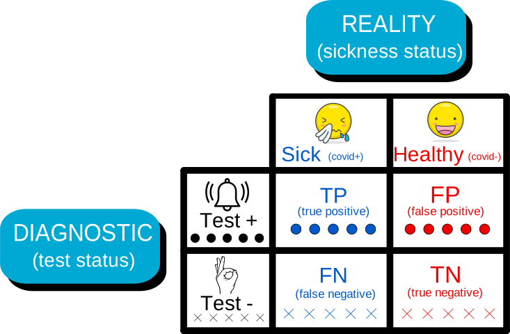{fig-alt="Illustration of TP, TN, FP, FN counts on a Covid-19 test example"}**Note**: the same color code is reused below.Red is for $\mathrm{N}$, blue for $\mathrm{P}$,crosses for a negative result,dots for a positive result.### The ratesLet $\pi_1\triangleq\mathbb{P}(Y=1)$and $\pi_0\triangleq1-\pi_1$.We call $\pi_1$ the **prevalence**.**Population rates**(probabilities, not counts):- $\mathrm{TPR}(t)=\mathbb{P}(\hat Y_t=1\mid Y=1)=\beta(t)$(**sensitivity**, **recall**):sick people correctly detected,- $\mathrm{FPR}(t)=\mathbb{P}(\hat Y_t=1\mid Y=0)=\alpha(t)$:healthy people wrongly flagged(the Type I error),- $\mathrm{TNR}(t)=\mathbb{P}(\hat Y_t=0\mid Y=0)=1-\alpha(t)$(**specificity**):healthy people correctly cleared,- $\mathrm{Precision}(t)=\mathbb{P}(Y=1\mid\hat Y_t=1)$:people declared positive who are really sick.By @eq-score, in terms of the scores:$$\begin{align*}\mathrm{TPR}(t)&=\mathbb{P}(T_1\ge t),\\\mathrm{FPR}(t)&=\mathbb{P}(T_0\ge t),\\\mathrm{TNR}(t)&=\mathbb{P}(T_0< t).\end{align*}$$The first three depend only onthe laws of $X_0,X_1$.**Precision** also depends on $\pi_0,\pi_1$(exact form in @thm-precision-formula below).This is why PR curves react to prevalenceand ROC curves do not.**Estimators.**In practice $t$, $\pi_1$ and the laws of $X_0,X_1$are unknown.Each rate is estimated on a labeled sampleby its empirical (plug-in) version:$$\begin{align*}\widehat{\mathrm{TPR}}(t) &=\frac{\mathrm{TP}(t)}{\mathrm{P}},\\\widehat{\mathrm{TNR}}(t) &=\frac{\mathrm{TN}(t)}{\mathrm{N}},\\\widehat{\mathrm{FPR}}(t) &=\frac{\mathrm{FP}(t)}{\mathrm{N}},\\\widehat{\mathrm{Precision}}(t)&=\frac{\mathrm{TP}(t)}{\hat{\mathrm{P}}_t}.\end{align*}$$Sweeping $t$ over $\mathbb{R}$turns these four numbersinto **curves**.That is the next section.## The ROC curveThe **receiver operating characteristic** (ROC) curvecomes from signal detection theory.This theory emerged from radar engineeringduring World War IIand was formalised by @peterson1954theory.The problem reads as follows: decide, from a noisy measurement,whether a target is presentor only background noise.A receiver declares "signal"when the measurement exceeds a threshold.The ROC curve records howthe detection rate and the false-alarm ratemove together as the threshold varies.This is the trade-off betweencatching true threatsand raising false alarms.In the language of this post,it is the power of the family $(\phi_t)_t$plotted against its Type I error.In such a context, one test gives one point;a family of tests gives a curve.:::: {#def-roc}# ROC curveLet $(\phi_t)_{t\in\mathbb{R}}$ be a family of tests(@def-family).For a threshold $t\in\mathbb{R}$,the **ROC operating point** is the pairof false and true positive rates,$$\begin{align*}\mathrm{FPR}(t) & = \mathbb{E}[\phi_t(X_0)] = \alpha(t),\\\mathrm{TPR}(t) & = \mathbb{E}[\phi_t(X_1)] = \beta(t).\end{align*}$$The **ROC curve** is the curvetraced by the operating pointas $t$ varies over $\mathbb{R}$:$$\{(\mathrm{FPR}(t), \mathrm{TPR}(t)) : t \in \mathbb{R}\}.$$::::For instance, for hard tests, $\phi_t=\mathbb{1}\{X\ge t\}$,this reads $\mathrm{FPR}(t)=\mathbb{P}(X_0\ge t)$and $\mathrm{TPR}(t)=\mathbb{P}(X_1\ge t)$.By @eq-score, in terms of the scores,$$\begin{align*}\mathrm{FPR}(t) & = \mathbb{P}(T_0\ge t),\\\mathrm{TPR}(t) & = \mathbb{P}(T_1\ge t).\end{align*}$$So the ROC curve of any familyis that of a plain threshold test on $(T_0,T_1)$.**Properties.**- Since FPR and TPR are probabilities,the curve lies in the unit square $[0,1]^2$.- By @eq-boundary, it goes from $(0,0)$(as $t\to+\infty$, nobody is flagged)to $(1,1)$(as $t\to-\infty$, everybody is flagged).- By @eq-nested, both coordinatesare non-increasing in $t$,so the curve is monotone.- If $T_0,T_1$ have atoms,the set of points has jumps.Several conventions exist to fill them: - **Straight segments**: randomize between the two neighboring tests. Every point on the segment is achievable by a randomized test, - **Steps**: a staircase (vertical, then horizontal), which makes no randomization assumption, - **No filling**: keep the isolated points. The choice changes the look of the curve, and the value of quantities computed from it (*e.g.,* the area under it). See @fig-gaussian-roc-interactive-samples below for a comparison on finite samples.### Properties#### ROC endpointsWe now treat the two extreme classifiers (that do **not** depend on a threshold):* **Always‑accept** (never reject): $\phi_{\text{acc}}(x)\equiv0$.* **Always‑reject** (always reject): $\phi_{\text{rej}}(x)\equiv1$.These are the two corner points of any ROC curve. The following lemma makes this precise.:::: {#lem-roc-endpoints}# ROC endpointsLet $(\phi_t)_{t\in\mathbb{R}}$ be a family of tests(@def-family).Then the ROC curve has the limiting endpoints$$\boxed{\lim_{t\to+\infty}\bigl(\mathrm{FPR}(t),\mathrm{TPR}(t)\bigr)=(0,0)}$$and$$\boxed{\lim_{t\to-\infty}\bigl(\mathrm{FPR}(t),\mathrm{TPR}(t)\bigr)=(1,1).}$$:::::::: {.proof-container}::: {.proof-header onclick="toggleProof('lem-roc-endpoints')"}[▶]{#proof-arrow-lem-roc-endpoints .proof-arrow} [Proof]{.proof-title}:::::: {#proof-content-lem-roc-endpoints .proof-content}By definition, for $j\in\{0,1\}$,$$\begin{align*}\mathrm{FPR}(t) &= \mathbb{E}[\phi_t(X_0)] = \alpha(t),\\\mathrm{TPR}(t) &= \mathbb{E}[\phi_t(X_1)] = \beta(t).\end{align*}$$**Step 1: limit as $t\to+\infty$.**By @eq-boundary, $\phi_t(X_j)\to0$ pointwise.Since $0\le\phi_t(X_j)\le1$,dominated convergence gives$$\mathbb{E}[\phi_t(X_j)]\to0,$$hence$$\boxed{\lim_{t\to+\infty} \bigl(\mathrm{FPR}(t),\mathrm{TPR}(t)\bigr) = (0,0).}$$**Step 2: limit as $t\to-\infty$.**By @eq-boundary, $\phi_t(X_j)\to1$ pointwise.Dominated convergence again gives$$\mathbb{E}[\phi_t(X_j)]\to1,$$hence$$\boxed{\lim_{t\to-\infty} \bigl(\mathrm{FPR}(t),\mathrm{TPR}(t)\bigr) = (1,1).}$$:::::::The point $(0,0)$ corresponds to a classifier that never declares a signal (no false‑positives, no true‑positives); the point $(1,1)$ corresponds to aclassifier that always declares a signal (maximal false‑positives and maximal true‑positives).Every ROC curve for a finite scoring rule must start at$(0,0)$ and end at $(1,1)$; the two extreme tests are precisely these endpoints, as formalized below:#### Extreme cases##### ROC curve for a perfect classifier:::: {#thm-perfect-separation}# ROC curve for a perfect classifierSuppose there exists a threshold $t^\star \in \mathbb{R}$ such that$$\mathbb{E}(\phi_{t^\star}(X_0)) = 0, \quad \mathbb{E}(\phi_{t^\star}(X_1)) = 1.$$Then,$$\boxed{\mathrm{FPR}(t^\star) = 0, \quad \mathrm{TPR}(t^\star) = 1,}$$and the ROC curve passes through the upper-left corner $(0,1)$ for $t^\star$.:::::::: {.proof-container}::: {.proof-header onclick="toggleProof('thm-perfect-separation')"}[▶]{#proof-arrow-thm-perfect-separation .proof-arrow} [Proof]{.proof-title}:::::: {#proof-content-thm-perfect-separation .proof-content}By definition, $\mathrm{FPR}(t^\star) = \mathbb{E}(\phi_{t^\star}(X_0))) = 0$ and $\mathrm{TPR}(t^\star) = \mathbb{E}(\phi_{t^\star}(X_1)) = 1$. Thus the threshold $t^\star$ yields the operating point $(0,1)$, representing perfect discrimination.:::::::##### ROC curve for an always-wrong classifier:::: {#cor-perfect-anti-separation}# ROC curve for an always-wrong classifierSuppose there exists a threshold $t^\star \in \mathbb{R}$ such that$$\mathbb{E}(\phi_{t^\star}(X_0)) = 1, \quad \mathbb{E}(\phi_{t^\star}(X_1)) = 0.$$Then,$$\boxed{\mathrm{FPR}(t^\star) = 1, \quad \mathrm{TPR}(t^\star) = 0,}$$and the ROC curve passes through the lower-right corner $(1,0)$.:::::::: {.proof-container}::: {.proof-header onclick="toggleProof('cor-perfect-anti-separation')"}[▶]{#proof-arrow-cor-perfect-anti-separation .proof-arrow} [Proof]{.proof-title}:::::: {#proof-content-cor-perfect-anti-separation .proof-content}By definition, $\mathrm{FPR}(t^\star) = \mathbb{E}(\phi_{t^\star}(X_0)) = 1$ and $\mathrm{TPR}(t^\star) = \mathbb{E}(\phi_{t^\star}(X_1)) = 0$. Thus the threshold $t^\star$ yields the operating point $(1,0)$, representing perfectly inverted discrimination.:::::::##### ROC curve under random guessing:::: {#thm-random-guessing}# ROC curve under random guessingSuppose $X_0 \stackrel{d}{=} X_1$. Then, for every $t \in \mathbb{R}$,$$\boxed{\mathrm{FPR}(t) = \mathrm{TPR}(t).}$$Consequently, the ROC curve lies on the diagonal line $u=v$ of the unit square.:::::::: {.proof-container}::: {.proof-header onclick="toggleProof('thm-random-guessing')"}[▶]{#proof-arrow-thm-random-guessing .proof-arrow} [Proof]{.proof-title}:::::: {#proof-content-thm-random-guessing .proof-content}Since $X_0 \stackrel{d}{=} X_1$, $\mathbb{P}(\phi_t(X_0) = 1) = \mathbb{E}(\phi_t(X_1))$ for every $t \in \mathbb{R}$, so $\mathrm{FPR}(t) = \mathrm{TPR}(t)$ for all $t$, and the ROC curve is included in the diagonal line.:::::::#### Monotonicity of ROC curvesMonotonicity is built into the definitionof a family of tests (@def-family).It is the **nested** condition @eq-nested:for all $x\in\mathbb{R}$,$$t_1<t_2\;\implies\;\phi_{t_1}(x)\ge\phi_{t_2}(x).$$It transfers to the ROC coordinates.It covers hard cut-offs $\mathbb{1}\{x\ge t\}$,scores $\mathbb{1}\{g(x)\ge t\}$and sigmoids $\sigma(g(x)-t)$.:::: {#thm-roc-monotonicity}# Monotonicity of ROC curvesLet $(\phi_t)_{t\in\mathbb{R}}$ be a family of tests(@def-family).Then for all $t_1<t_2$,$$\begin{align*}\mathrm{TPR}(t_1)&\ge\mathrm{TPR}(t_2),\\\mathrm{FPR}(t_1)&\ge\mathrm{FPR}(t_2).\end{align*}$$In words:both rates are non-increasingas the threshold increases.:::::::: {.proof-container}::: {.proof-header onclick="toggleProof('thm-roc-monotonicity')"}[▶]{#proof-arrow-thm-roc-monotonicity .proof-arrow} [Proof]{.proof-title}:::::: {#proof-content-thm-roc-monotonicity .proof-content}Recall that$$\begin{align*}\mathrm{TPR}(t)&=\mathbb{E}[\phi_t(X_1)]=\beta(t),\\\mathrm{FPR}(t)&=\mathbb{E}[\phi_t(X_0)]=\alpha(t).\end{align*}$$Fix $t_1<t_2$.By @eq-nested, pointwise in $x$,$$\phi_{t_1}(x)\ge\phi_{t_2}(x).$$Hence, for every outcome $\omega$ and for $j\in\{0,1\}$,$$\phi_{t_1}(X_j(\omega))\ge\phi_{t_2}(X_j(\omega)).$$Both variables are bounded in $[0,1]$,so their expectations exist.Expectation preserves order, so$$\mathbb{E}[\phi_{t_1}(X_j)]\ge\mathbb{E}[\phi_{t_2}(X_j)],\qquad j\in\{0,1\}.$$Taking $j=1$ gives$\mathrm{TPR}(t_1)\ge\mathrm{TPR}(t_2)$.Taking $j=0$ gives$\mathrm{FPR}(t_1)\ge\mathrm{FPR}(t_2)$.:::::::##### Invariance of ROC curves under increasing transformsLet $g:\mathbb{R}\to\mathbb{R}$be a **strictly increasing bijection**,and set $Z_j=g(X_j)$, $j\in\{0,1\}$ and $Z=g(X)$.We relabel the familyto act on the transformed data:$$\widetilde\phi_t(z)\triangleq\phi_{g^{-1}(t)}\bigl(g^{-1}(z)\bigr),\qquad t,z\in\mathbb{R}.$$ {#eq-transformed-family}Its rates on $Z$ are$$\begin{align*}\mathrm{FPR}_{Z}(t)&=\mathbb{E}[\widetilde\phi_t(Z_0)],\\\mathrm{TPR}_{Z}(t)&=\mathbb{E}[\widetilde\phi_t(Z_1)].\end{align*}$$:::: {#thm-roc-bijective-transform}# Invariance under strictly increasing transformsLet $(\phi_t)_{t\in\mathbb{R}}$ be a family of tests(@def-family),and $g$ a strictly increasing bijection.Then:1. $(\widetilde\phi_t)_{t\in\mathbb{R}}$is a family of tests (@def-family),2. for every $t\in\mathbb{R}$,$$\boxed{\begin{aligned}\mathrm{FPR}_{Z}(t)&=\mathrm{FPR}_X\bigl(g^{-1}(t)\bigr),\\\mathrm{TPR}_{Z}(t)&=\mathrm{TPR}_X\bigl(g^{-1}(t)\bigr).\end{aligned}}$$3. the two ROC curves coincide:$$\{(\mathrm{FPR}_{Z}(t),\mathrm{TPR}_{Z}(t)):t\in\mathbb{R}\}=\{(\mathrm{FPR}_X(s),\mathrm{TPR}_X(s)):s\in\mathbb{R}\}.$$Only the labelling of the pointsby a threshold changes,through the increasing map $t\mapsto g^{-1}(t)$.:::::::: {.proof-container}::: {.proof-header onclick="toggleProof('thm-roc-bijective-transform')"}[▶]{#proof-arrow-thm-roc-bijective-transform .proof-arrow} [Proof]{.proof-title}:::::: {#proof-content-thm-roc-bijective-transform .proof-content}**Step 1: $\widetilde\phi$ is a family of tests.**The map $g^{-1}$ is a strictly increasing bijectionof $\mathbb{R}$, hence continuous,with $g^{-1}(t)\to\pm\infty$ as $t\to\pm\infty$.Fix $z\in\mathbb{R}$ and set $x=g^{-1}(z)$.- *Nested.*If $t_1<t_2$, then $g^{-1}(t_1)<g^{-1}(t_2)$.By @eq-nested,$\widetilde\phi_{t_1}(z)\ge\widetilde\phi_{t_2}(z)$.- *Left-continuous.*If $u\uparrow t$, then $g^{-1}(u)\uparrow g^{-1}(t)$strictly from below.By @eq-left-cont,$\widetilde\phi_u(z)\to\widetilde\phi_t(z)$.- *Boundary.*By @eq-boundary and the limits of $g^{-1}$,$\widetilde\phi_t(z)\to1$ as $t\to-\infty$and $\to0$ as $t\to+\infty$.**Step 2: pointwise identity.**Take $z=g(x)$. Then $g^{-1}(z)=x$, so$$\widetilde\phi_t\bigl(g(x)\bigr)=\phi_{g^{-1}(t)}(x).$$ {#eq-pointwise-id}**Step 3: rates.**Since $Z_j=g(X_j)$, @eq-pointwise-id gives$\widetilde\phi_t(Z_j)=\phi_{g^{-1}(t)}(X_j)$as random variables.Taking expectations,$$\begin{align*}\mathrm{FPR}_{g(X)}(t)&=\mathbb{E}[\phi_{g^{-1}(t)}(X_0)]=\mathrm{FPR}_X\bigl(g^{-1}(t)\bigr),\\\mathrm{TPR}_{g(X)}(t)&=\mathbb{E}[\phi_{g^{-1}(t)}(X_1)]=\mathrm{TPR}_X\bigl(g^{-1}(t)\bigr).\end{align*}$$**Step 4: curves.**Since $g^{-1}$ is a bijection of $\mathbb{R}$,$s=g^{-1}(t)$ runs over all of $\mathbb{R}$as $t$ does.So both sets of points are the same.:::::::**Special cases and scores.**- For $\phi_t(x)=\mathbb{1}\{x\ge t\}$,$$\widetilde\phi_t(z)=\mathbb{1}\{g^{-1}(z)\ge g^{-1}(t)\}=\mathbb{1}\{z\ge t\}.$$So the cut-off on $Z=g(X)$has the same ROC curve as the cut-off on $X$.- In terms of @thm-create-test,the score of $\widetilde\phi$is $g(T_j)$:$\mathbb{P}(g(T_j)\ge t)=\mathbb{P}(T_j\ge g^{-1}(t))$.- Only the *ranking* of scores matters,not their scale.#### Symmetries of ROC curvesReversing the decision ruleand/or swapping the class labelsacts on the ROC curveas an exact affine reflectionof the unit square.Write $\mathcal{C}$ for the ROC curveof a family $(\phi_t)_t$ (@def-roc).Consider the three maps of the square:$$\begin{align*}R(x,y)&=(1-x,\,1-y),\\S(x,y)&=(y,\,x),\\R\circ S\,(x,y)&=(1-y,\,1-x).\end{align*}$$They are the central reflection about $(\tfrac12,\tfrac12)$,the reflection about $y=x$,and the reflection about $y=1-x$.**Why prevalence plays no role.**$\mathrm{FPR}$ and $\mathrm{TPR}$ depend only onthe laws of $X_0$ and $X_1$,never on $\pi_0,\pi_1$.So all three symmetriesare statements about these two laws.##### Test reversalKeep the labels, reverse the rule.Raising the threshold must stillmake the test *less* positive,so we reindex and use right limits:$$\phi^{\mathrm{rev}}_t(x)\triangleq1-\phi_{(-t)+}(x),\qquad t\in\mathbb{R}.$$ {#eq-reversed-family}The operating point is sent to$$\boxed{\binom{\mathrm{FPR}(t)}{\mathrm{TPR}(t)}\longmapsto\binom{1-\mathrm{FPR}(t)}{1-\mathrm{TPR}(t)}}$$(exactly so when $\alpha,\beta$ are continuous;otherwise see the proof).:::: {#thm-roc-threshold-reversal}# Central symmetryLet $(\phi_t)_{t\in\mathbb{R}}$ be a family of tests(@def-family). Then:1. $(\phi^{\mathrm{rev}}_t)_{t\in\mathbb{R}}$is a family of tests,2. its ROC curve is $R(\mathcal{C})$,the central reflection of $\mathcal{C}$about $(\tfrac12,\tfrac12)$.:::::::: {.proof-container}::: {.proof-header onclick="toggleProof('thm-roc-threshold-reversal')"}[▶]{#proof-arrow-thm-roc-threshold-reversal .proof-arrow} [Proof]{.proof-title}:::::: {#proof-content-thm-roc-threshold-reversal .proof-content}**Step 1: a family of tests.**Fix $x$ and put $s=-t$.- *Nested.*If $t_1<t_2$, then $-t_1>-t_2$.By @eq-nested,$\phi_{(-t_1)+}(x)\le\phi_{(-t_2)+}(x)$,so $\phi^{\mathrm{rev}}_{t_1}(x)\ge\phi^{\mathrm{rev}}_{t_2}(x)$.- *Left-continuous.*If $u\uparrow t$, then $-u\downarrow -t$,so $\phi_{(-u)+}(x)\to\phi_{(-t)+}(x)$.- *Boundary.*As $t\to-\infty$, $-t\to+\infty$ and$\phi_{(-t)+}(x)\to0$, so $\phi^{\mathrm{rev}}_t(x)\to1$.Symmetrically, $\phi^{\mathrm{rev}}_t(x)\to0$as $t\to+\infty$.**Step 2: rates.**By @thm-create-test,$\mathbb{E}[\phi_{s+}(X_j)]=\alpha(s+)$or $\beta(s+)$. Hence$$\begin{align*}\mathrm{FPR}^{\mathrm{rev}}(t)&=1-\alpha\bigl((-t)+\bigr),\\\mathrm{TPR}^{\mathrm{rev}}(t)&=1-\beta\bigl((-t)+\bigr).\end{align*}$$**Step 3: curve.**With $s=-t$, the operating points are$R\bigl(\alpha(s+),\beta(s+)\bigr)$, $s\in\mathbb{R}$.These are the right-limit points of $\mathcal{C}$.At a jump, they are the endpoints of the filled segment,and $R$ maps segments to segments.Hence the ROC curve of the reversed family is $R(\mathcal{C})$.If $\alpha,\beta$ are continuous,$\alpha(s+)=\alpha(s)$ and this is just$(\mathrm{FPR},\mathrm{TPR})\mapsto(1-\mathrm{FPR},1-\mathrm{TPR})$.:::::::##### Class label swapKeep the rule, swap the labels:$Y'=1-Y$, so $X_0'=X_1$ and $X_1'=X_0$.The operating point is sent to$$\boxed{\binom{\mathrm{FPR}(t)}{\mathrm{TPR}(t)}\longmapsto\binom{\mathrm{TPR}(t)}{\mathrm{FPR}(t)}.}$$:::: {#thm-roc-class-swap}# Main-diagonal symmetryLet $(\phi_t)_{t\in\mathbb{R}}$ be a family of tests(@def-family).With the labels swapped and the family unchanged,the ROC curve is $S(\mathcal{C})$,the reflection of $\mathcal{C}$about the diagonal $y=x$.:::::::: {.proof-container}::: {.proof-header onclick="toggleProof('thm-roc-class-swap')"}[▶]{#proof-arrow-thm-roc-class-swap .proof-arrow} [Proof]{.proof-title}:::::: {#proof-content-thm-roc-class-swap .proof-content}The family is unchanged,so it is still a family of tests.Only the roles of $X_0,X_1$ are exchanged:$$\begin{align*}\mathrm{FPR}'(t)&=\mathbb{E}[\phi_t(X_0')]=\mathbb{E}[\phi_t(X_1)]=\mathrm{TPR}(t),\\\mathrm{TPR}'(t)&=\mathbb{E}[\phi_t(X_1')]=\mathbb{E}[\phi_t(X_0)]=\mathrm{FPR}(t).\end{align*}$$So $(\mathrm{FPR}',\mathrm{TPR}')(t)=S(\mathrm{FPR},\mathrm{TPR})(t)$for every $t$.$S$ is affine, so it also maps filled segments to filled segments.:::::::##### Label swap with test reversalSwap the labels **and** reverse the rule(@eq-reversed-family).The operating point is sent to$$\boxed{\binom{\mathrm{FPR}(t)}{\mathrm{TPR}(t)}\longmapsto\binom{1-\mathrm{TPR}(t)}{1-\mathrm{FPR}(t)}.}$$:::: {#thm-roc-class-inversion}# Anti-diagonal symmetryLet $(\phi_t)_{t\in\mathbb{R}}$ be a family of tests(@def-family).With the labels swapped and the rule reversed,the ROC curve is $(R\circ S)(\mathcal{C})$,the reflection of $\mathcal{C}$about the anti-diagonal $y=1-x$.:::::::: {.proof-container}::: {.proof-header onclick="toggleProof('thm-roc-class-inversion')"}[▶]{#proof-arrow-thm-roc-class-inversion .proof-arrow} [Proof]{.proof-title}:::::: {#proof-content-thm-roc-class-inversion .proof-content}Apply @thm-roc-threshold-reversalto the family $(\phi_t)$,then @thm-roc-class-swapto the reversed family(a family of tests by Step 1).The two reflections compose to$$R\circ S\,(x,y)=(1-y,\,1-x).$$Concretely, with $s=-t$,$\mathrm{FPR}'(t)=1-\beta(s+)$and $\mathrm{TPR}'(t)=1-\alpha(s+)$.Since $R\circ S=S\circ R$,the order of the two operations does not matter.:::::::**Consequences.**- Reversing a worse-than-chance test makes it better than chance (reflection about $(\tfrac12,\tfrac12)$).- A curve symmetric under $S$ is unchanged by label swapping.- The curve of any "worse than chance" familycan be improved by reversing it.##### Summary and visualization::: {style="font-size:90%; overflow-x:auto; margin: 1em 0;"} | Transformation | FPR$'$ / TPR$'$ | Geometry | |---|---|---| | Test reversal | $1-\mathrm{FPR}$ / $1-\mathrm{TPR}$ | Central symmetry, center $(0.5,0.5)$ | | Label swap | $\mathrm{TPR}$ / $\mathrm{FPR}$ | Main diagonal $y=x$ | | Reversal + swap | $1-\mathrm{TPR}$ / $1-\mathrm{FPR}$ | Anti-diagonal $y=1-x$ |: Transformations of the ROC operating point. Reversal: $X<t \leftrightarrow X\ge t$; label swap: $Y=0\leftrightarrow Y=1$. {#tbl-roc-transformations .striped .hover}:::These three transformations creat reflected copy shape. As noted above, none of them depends on the class prevalence $\pi_1$.You can verify this directly with the interactive below.**Interactive ROC curve exploration.** The visualization below illustrates these properties for a Gaussian model $X\mid Y=0\sim\mathcal N(0,1)$, $X\mid Y=1\sim\mathcal N(1,2^2)$. Use the **Threshold** slider to move along the ROC curve and watch the operating point change; the **Prevalence ($\pi_1$)** slider confirms that the ROC curve itself is unaffected by class imbalance, however that slider is moved. The plot also shows the reversed-rule and class-inverted curves described above.::: {#fig-gaussian-symmetric-roc}```{=html}<div id="gaussian-symmetric-roc-interactive" class="gaussian-symmetric-roc-interactive" style="display:flex; gap:10px; align-items:stretch; flex-wrap:wrap; width:100%; max-width:700px; margin:0 auto; overflow-x:auto; font-family:'Inter', -apple-system, 'Segoe UI', Helvetica, Arial, sans-serif;"> <div class="gaussian-symmetric-roc-controls" style="display:flex; flex-direction:column; justify-content:center; min-width:150px; flex:0 0 150px; border:1px solid rgba(0,0,0,0.15); border-radius:8px; padding:8px; font-size:9.5px; background:rgba(0,0,0,0.02);"> </div> <div class="gaussian-symmetric-roc-plot" style="flex:1 1 340px; min-width:340px; display:flex; align-items:center; justify-content:center;"> </div></div><script type="module" src="gaussian_symmetric_roc.js"></script>```**ROC curve under symmetry transformations**:::### ROC curves for common distributionsBelow we summarize the ROC curves for classic location-scale distributions, along with the exponential case.Throughout, we assume that $Z_0, Z_1$ are independent and identically distributed with a common continuous CDF $F$. The tests considered here are written as $\mathbb{1}(X \ge t)$.We define the location-scale variables as:$$\begin{align*}X_0 & = \sigma_0 Z_0 + \mu_0,\\X_1 & = \sigma_1 Z_1 + \mu_1,\end{align*}$$where $\sigma_0 > 0$ and $\sigma_1 > 0$ are the scale parameters, and $\mu_0, \mu_1 \in \mathbb{R}$ are the location parameters. We use the following notation:- $\Delta = (\mu_1 - \mu_0) / \sigma_1$ (standardized separation)- $\rho = \sigma_0 / \sigma_1 > 0$ (scale ratio)- $\Phi(z) = \int_{-\infty}^z \frac{1}{\sqrt{2\pi}} e^{-u^2/2} \, du$ (standard Gaussian CDF)- $\Psi(z) = \frac{1}{2} + \frac{1}{\pi} \arctan(z)$ (Standard Cauchy CDF) and $\Psi^{-1}(u) = \tan\left(\pi\left(u - \frac{1}{2}\right)\right)$.- $[x]_0^1 = \max(0, \min(1, x))$ (clipping function)- $(x)_+= \max(0,x)$::: {style="font-size:90%; margin: 1em 0;"}| **Law of $Z$** | **$F(z)$** | **$\mathrm{TPR}(u)$, $u=\mathrm{FPR}$** ||:---------------|:-----------|:--------------------------------------|| **Gaussian** | $\Phi(z)$ | $\Phi\!\left(\Delta+\rho\Phi^{-1}(u)\right)$ || **Cauchy** | $\Psi(z)$ | $\Psi\left(\Delta + \rho \Psi^{-1}(u)\right)$ || **Logistic** | $\frac{1}{1+e^{-z}}$ | $\frac{e^\Delta u^\rho}{e^\Delta u^\rho+(1-u)^\rho}$ || **Uniform** $(-\tfrac12,\tfrac12)$ | $[z+\frac12]_0^1$ | $[\Delta+\frac{1-\rho}{2}+\rho u]_0^1$ || **Gumbel** | $e^{-e^{-z}}$ | $1-e^{\left[-e^\Delta(-\ln(1-u))^\rho\right]}$ || **Exp.** | $(1-e^{-z})_+$ | $\min(e^\Delta u^\rho,1)$ |: ROC curves for common distributions {#tbl-distributions .striped .hover}:::**Where the table comes from.** All the rows follow from a single identity (@thm-location-scale-roc): for $X_y=\sigma_yZ_y+\mu_y$ with $Z_0,Z_1$ i.i.d. with CDF $F$,$$\mathrm{TPR}\!=\!1\!-\!F\bigl(\rho\,F^{-1}(1\!-\!\mathrm{FPR})\!-\!\Delta\bigr),$$which simplifies to $\mathrm{TPR}=F\bigl(\Delta+\rho\,F^{-1}(\mathrm{FPR})\bigr)$ when $F$ is symmetric (@cor-symmetric-roc). The statements, the proofs, and the row-by-row computations (Gaussian, Cauchy, Logistic, Uniform, Gumbel, Exponential) are collected in [Appendix A](#sec-app-roc).**Visualization**The widget below lets you explore @thm-location-scale-roc interactively for the distribution described in @tbl-distributions.Use the sliders on the left to set $\mu_0,\sigma_0$ (healthy class) and $\mu_1,\sigma_1$ (sick class), and drag the **Threshold** slider to move $t$.- The **middle panel** shows the two population densities plotted vertically: $X_1$ (sick) on the left in blue, $X_0$ (healthy) on the right in red. The horizontal black line marks the current threshold $t$; the darker-shaded region of each density is $\{X<t\}$ (the portion of that class predicted *negative* under the rule $\hat{Y}_t=\mathbb{1}\{X\ge t\}$) while the lighter region above the line is predicted *positive*.- The **right panel** shows the theoretical ROC curve for the current $(\mu_0,\sigma_0,\mu_1,\sigma_1)$, with the dashed diagonal as the random-guessing reference (@thm-random-guessing) and a marker at the operating point $(\mathrm{FPR}(t),\mathrm{TPR}(t))$ corresponding to the threshold you've selected, so you can see exactly which point on the curve a given threshold produces, and watch the curve itself deform as you change the means, standard deviations, or their ratio $\rho=\tfrac{\sigma_0}{\sigma_1}$.The title above the plot reports the current $\Delta=\tfrac{(\mu_1-\mu_0)}{\sigma_1}$, $\rho = \tfrac{\sigma_0}{\sigma_1}$.::: {#fig-gaussian-roc-interactive}```{=html}<div id="gaussian-roc-interactive" class="gaussian-roc-interactive" style="display:flex; gap:10px; align-items:stretch; flex-wrap:nowrap; width:100%; max-width: min(895px, 100%); margin:0 auto; overflow-x:auto; font-family:'Inter', -apple-system, 'Segoe UI', Helvetica, Arial, sans-serif;"> <div class="gaussian-roc-controls" style="display:flex; flex-direction:column; justify-content:center; min-width:125px; flex:0 0 115px; border:1px solid rgba(0,0,0,0.15); border-radius:8px; padding:6px; font-size:9px; background:rgba(0,0,0,0.02);"> </div> <div class="gaussian-roc-plot" style="flex:1 1 auto; min-width:260px; display:flex; align-items:center; justify-content:center;"> </div></div><script type="module" src="gaussian_roc_interactive.js"></script>```**ROC curve for classic distributions**:::**Note**: Visually, the TPR is the ratio of the light blue area over the full blue area on the left, while the FPR is the ratio of the light red area over the full red area (right).**Interpretation**$\Delta=(\mu_1-\mu_0)/\sigma_1$ measures the (scale-standardized) separation between $X_0$ and $X_1$; $\rho=\sigma_0/\sigma_1$ compares their spread. Together they set the difficulty and shape of the ROC curve.* **$\rho=1$:** the usual equal-scale model, $\mathrm{TPR}=F(\Delta+F^{-1}(\mathrm{FPR}))$ for symmetric $F$, e.g., the binormal case $\mathrm{TPR}=\Phi(\Delta+\Phi^{-1}(\mathrm{FPR}))$.* **$\Delta=0,\ \rho=1$:** $X_0\stackrel{d}{=}X_1$, and the ROC curve is the diagonal (random guessing). Note $\Delta=0$ alone is *not* enough when $\rho\ne1$: equal location with unequal scale still separates the classes, via spread rather than location.* **$\rho\ne1$:** the curve need not be symmetric about the anti-diagonal or concave everywhere, if $\rho<1$ (sick population more dispersed), the curve can dip toward the diagonal near one corner before rising, a non-concave S-shape sometimes seen in real assay data.* **$\Delta\to\infty$** (fixed $\rho$): the classes separate perfectly, and the curve approaches the ideal curve through $(0,1)$.Now we illustrate the empirical counterpart, when one samples elements from the distributions but without access to the true densities.::: {#fig-gaussian-roc-interactive-samples}```{=html}<div id="sampling-roc-interactive" class="sampling-roc-interactive" style="display:flex; gap:10px; align-items:stretch; flex-wrap:nowrap; width:100%; max-width: min(895px, 100%); margin:0 auto; overflow-x:auto; font-family:'Inter', -apple-system, 'Segoe UI', Helvetica, Arial, sans-serif;"> <div class="sampling-roc-controls" style="display: flex; flex-direction:column; justify-content: center; min-width:130px; flex:0 0 120px; border:1px solid rgba(0,0,0,0.15); border-radius:8px; padding:6px; font-size:9px; background:rgba(0,0,0,0.02);"> </div> <div class="sampling-roc-plot" style="flex:1 1 auto; min-width:260px; display:flex; align-items:center; justify-content:center;"> </div></div><script type="module" src="roc_sampling_explorer.js"></script>```**Empirical counterpart of ROC curve for classic distributions.**:::ROC curves are commonly displayed with stepwise (vertical and horizontal) segments, but using affine interpolation between points provides a more informative visualization.In particular, the affine approach better reveals non-concavities in the curve, offering clearer insights into classifier performance and highlighting suboptimal decision thresholds (as explained below). Smooth interpolation distinguishes subtle variations in behavior that would otherwise be obscured by the sharp transitions of stepwise plots.#### ROC curves and Neyman-PearsonSo far, a family $(\phi_t)_t$ gave one ROC curve.Now we ask the converse question:**how good can a ROC curve be?**We need two tools:randomization, and the likelihood ratio.##### Randomized mixturesLet $\mathcal{T}$ be the set of all measurable tests$\phi:\mathbb{R}\to[0,1]$.For $\phi\in\mathcal{T}$, write$$\begin{align*}\mathrm{FPR}(\phi)&=\mathbb{E}[\phi(X_0)],\\\mathrm{TPR}(\phi)&=\mathbb{E}[\phi(X_1)].\end{align*}$$This extends the rates of $\phi_t$to any single test.:::: {#thm-roc-randomization}# Randomized mixturesLet $\phi,\phi'\in\mathcal{T}$with operating points$P=(\mathrm{FPR}(\phi),\mathrm{TPR}(\phi))$and $P'=(\mathrm{FPR}(\phi'),\mathrm{TPR}(\phi'))$.For $\lambda\in[0,1]$, set$$\phi_\lambda\triangleq\lambda\phi+(1-\lambda)\phi'.$$Then $\phi_\lambda\in\mathcal{T}$, and$$\begin{align*}\mathrm{FPR}(\phi_\lambda)&=\lambda\,\mathrm{FPR}(\phi)+(1-\lambda)\,\mathrm{FPR}(\phi'),\\\mathrm{TPR}(\phi_\lambda)&=\lambda\,\mathrm{TPR}(\phi)+(1-\lambda)\,\mathrm{TPR}(\phi').\end{align*}$$As $\lambda$ goes from $0$ to $1$,the operating point sweeps the segment $[P,P']$.:::::::: {.proof-container}::: {.proof-header onclick="toggleProof('thm-roc-randomization')"}[▶]{#proof-arrow-thm-roc-randomization .proof-arrow} [Proof]{.proof-title}:::::: {#proof-content-thm-roc-randomization .proof-content}$\phi_\lambda$ is measurable with values in $[0,1]$,as a convex combination of such maps.Linearity of expectation gives both identities.The map $\lambda\mapsto\lambda P+(1-\lambda)P'$parametrizes $[P,P']$.:::::::**Interpretation.**$\phi_\lambda(x)$ is the probabilityof declaring positive when we flip a coin:use $\phi$ with probability $\lambda$,$\phi'$ otherwise.This justifies the *straight-segment* conventionfor filling jumps of a ROC curve:two neighboring tests of a familycan always be mixed.Let $\mathcal{R}\triangleq\{(\mathrm{FPR}(\phi),\mathrm{TPR}(\phi)):\phi\in\mathcal{T}\}$be the **attainable region**.**Properties of $\mathcal{R}$.**- It is **convex**(@thm-roc-randomization).- It contains $(0,0)$ and $(1,1)$(take $\phi\equiv0$ and $\phi\equiv1$).- It is symmetric under $R$, the central symmetry of center $(1/2, 1/2)$(take $1-\phi$): $R(\mathcal{R})=\mathcal{R}$.Hence only the **upper boundary** of $\mathcal{R}$ matters.Any point below it is matched or beatenby mixing two tests on the boundary.The next theorem identifies this boundary.##### The likelihood-ratio testAssume $X_0,X_1$ have densities $f_0,f_1$with respect to a common $\sigma$-finite measure $\mu$,and $f_0>0$ $\mu$-a.e.Define the **likelihood ratio**$$L(x)\triangleq\frac{f_1(x)}{f_0(x)}\in[0,\infty).$$For $k\in[0,\infty]$ and $\gamma\in[0,1]$, set$$\phi^{\mathrm{LR}}_{k,\gamma}(x)=\begin{cases}1 & L(x)>k,\\\gamma & L(x)=k,\\0 & L(x)<k.\end{cases}$$:::: {#lem-np-level}# Exact levelFor every $\alpha\in[0,1]$there exist $k_\alpha\in[0,\infty]$ and $\gamma_\alpha\in[0,1]$such that$$\mathrm{FPR}\bigl(\phi^{\mathrm{LR}}_{k_\alpha,\gamma_\alpha}\bigr)=\alpha.$$We write $\phi^{\mathrm{LR}}_\alpha\triangleq\phi^{\mathrm{LR}}_{k_\alpha,\gamma_\alpha}$.:::::::: {.proof-container}::: {.proof-header onclick="toggleProof('lem-np-level')"}[▶]{#proof-arrow-lem-np-level .proof-arrow} [Proof]{.proof-title}:::::: {#proof-content-lem-np-level .proof-content}Let $H(k)\triangleq\mathbb{P}(L(X_0)>k)$.It is non-increasing and right-continuous,with $H(\infty)=0$ and $H(0)\le1$.Set $k_\alpha\triangleq\inf\{k\ge0:H(k)\le\alpha\}$.- If $k_\alpha=\infty$, then $\alpha=0$and $\phi^{\mathrm{LR}}_\alpha\equiv0$ ($\mu$-a.e., since $f_0>0$).- Otherwise, right-continuity gives $H(k_\alpha)\le\alpha\le H(k_\alpha-)$,and $H(k_\alpha-)-H(k_\alpha)=\mathbb{P}(L(X_0)=k_\alpha)$.If this probability is $0$, take $\gamma_\alpha=0$.If not, take$$\gamma_\alpha=\frac{\alpha-H(k_\alpha)}{\mathbb{P}(L(X_0)=k_\alpha)}\in[0,1].$$- In both cases, $\mathbb{E}[\phi^{\mathrm{LR}}_\alpha(X_0)] =H(k_\alpha)+\gamma_\alpha\,\mathbb{P}(L(X_0)=k_\alpha)=\alpha$.::::::::::: {#thm-neyman-pearson}# Neyman–Pearson optimalityFor every $\alpha\in[0,1]$,$\phi^{\mathrm{LR}}_\alpha$ has the highesttrue positive rate among all tests of level $\alpha$:$$\boxed{\mathrm{TPR}(\phi^{\mathrm{LR}}_\alpha)=\sup\bigl\{\mathrm{TPR}(\phi):\phi\in\mathcal{T},\ \mathrm{FPR}(\phi)=\alpha\bigr\}.}$$Set $\beta^\star(\alpha)\triangleq\mathrm{TPR}(\phi^{\mathrm{LR}}_\alpha)$. Then:1. the point $(\alpha,\beta^\star(\alpha))$lies on or above every operating point $(\mathrm{FPR}(\phi),\mathrm{TPR}(\phi))$,$\phi\in\mathcal{T}$ (**upper envelope**),2. $\beta^\star$ is **concave** on $[0,1]$.:::::::: {.proof-container}::: {.proof-header onclick="toggleProof('thm-neyman-pearson')"}[▶]{#proof-arrow-thm-neyman-pearson .proof-arrow} [Proof]{.proof-title}:::::: {#proof-content-thm-neyman-pearson .proof-content}**Step 1: optimality at level $\alpha$.**Fix $\phi\in\mathcal{T}$ with $\mathrm{FPR}(\phi)=\alpha$.Write $\phi^\star\triangleq\phi^{\mathrm{LR}}_\alpha$and $k\triangleq k_\alpha$.*Case $k<\infty$.*For $x\in\mathbb{R}$, set$$D(x)\triangleq\bigl(\phi^\star(x)-\phi(x)\bigr)\bigl(f_1(x)-k\,f_0(x)\bigr).$$Since $f_0(x)>0$, we have$f_1(x)-k f_0(x)=f_0(x)\bigl(L(x)-k\bigr)$,so its sign is that of $L(x)-k$. Hence:- if $L(x)>k$: $\phi^\star(x)=1\ge\phi(x)$and $f_1(x)-kf_0(x)>0$,- if $L(x)<k$: $\phi^\star(x)=0\le\phi(x)$and $f_1(x)-kf_0(x)<0$,- if $L(x)=k$: $f_1(x)-kf_0(x)=0$.In every case $D(x)\ge0$, for $\mu$-almost every $x$.All terms are integrable ($0\le\phi,\phi^\star\le1$,$f_0,f_1$ are densities, $k<\infty$), so$$\begin{align*}0&\le\int D(x)\,d\mu(x)\\&=\int\bigl(\phi^\star(x)-\phi(x)\bigr)f_1(x)\,d\mu(x)\\&\quad-k\int\bigl(\phi^\star(x)-\phi(x)\bigr)f_0(x)\,d\mu(x)\\&=\bigl(\mathrm{TPR}(\phi^\star)-\mathrm{TPR}(\phi)\bigr)-k\bigl(\mathrm{FPR}(\phi^\star)-\mathrm{FPR}(\phi)\bigr).\end{align*}$$Both tests have level $\alpha$,so the last bracket is $\alpha-\alpha=0$.Hence $\mathrm{TPR}(\phi^\star)\ge\mathrm{TPR}(\phi)$.*Case $k=\infty$.*Then $\alpha=0$ and $\phi^\star(x)=0$ for all $x$,so $\mathrm{TPR}(\phi^\star)=0$.Since $\mathrm{FPR}(\phi)=\int\phi(x)f_0(x)\,d\mu(x)=0$and $f_0(x)>0$,we get $\phi(x)=0$ for $\mu$-almost every $x$.Hence $\mathrm{TPR}(\phi)=\int\phi(x)f_1(x)\,d\mu(x)=0$.**Step 2: envelope.**Step 1 applies to every $\phi\in\mathcal{T}$,at its own level $\alpha=\mathrm{FPR}(\phi)$.Hence, for all $\phi\in\mathcal{T}$,$$\mathrm{TPR}(\phi)\le\beta^\star\bigl(\mathrm{FPR}(\phi)\bigr).$$**Step 3: concavity.**Take $\alpha_1,\alpha_2\in[0,1]$ and $\lambda\in[0,1]$.Set $\alpha\triangleq\lambda\alpha_1+(1-\lambda)\alpha_2$and, for $x\in\mathbb{R}$,$$\psi(x)\triangleq\lambda\,\phi^{\mathrm{LR}}_{\alpha_1}(x)+(1-\lambda)\,\phi^{\mathrm{LR}}_{\alpha_2}(x).$$Then $\psi\in\mathcal{T}$, and by @thm-roc-randomization,$$\begin{align*}\mathrm{FPR}(\psi)&=\lambda\alpha_1+(1-\lambda)\alpha_2=\alpha,\\\mathrm{TPR}(\psi)&=\lambda\,\beta^\star(\alpha_1)+(1-\lambda)\,\beta^\star(\alpha_2).\end{align*}$$Since $\psi$ has level $\alpha$,Step 1 gives $\mathrm{TPR}(\psi)\le\beta^\star(\alpha)$.That is,$$\beta^\star\bigl(\lambda\alpha_1+(1-\lambda)\alpha_2\bigr)\ge\lambda\,\beta^\star(\alpha_1)+(1-\lambda)\,\beta^\star(\alpha_2).$$:::::::**Any score that ranks like $L$ is optimal.**If $g=h\circ L$ with $h$ strictly increasing,then $\{g\ge t\}$ is of the form $\{L\ge s\}$ or $\{L>s\}$.So $\mathbb{1}\{g(x)\ge t\}\in\{\phi_s(x),\phi_{s+}(x)\}$:same operating points, same curve.A model is judged on how well it *ranks* by $L$,not on its scale.##### Likelihood-ratio tests for the Gaussian exampleLet $X\mid Y=0\sim\mathcal N(0,1)$ and $X\mid Y=1\sim\mathcal N(1,4)$, with $\Phi$ the standard normal CDF.**1. Likelihood-ratio (Neyman–Pearson) test**The densities are$$f_0(x)=\frac{1}{\sqrt{2\pi}}e^{-x^{2}/2},\qquadf_1(x)=\frac{1}{2\sqrt{2\pi}}e^{-(x-1)^{2}/8}.$$Hence, the log-likelihood ratio is$$\begin{align*}\ell^{LR}(x) & =\log\frac{f_1(x)}{f_0(x)}\\ & =\frac{3}{8}x^{2}+\frac14x-\frac18-\log 2 \\ & =\frac38\!\Bigl(x+\frac13\Bigr)^{2}-\frac16-\log 2 .\end{align*}$$so the threshold-$\lambda$ test defined as $\mathbb{1}(\ell^{LR}(x) \ge \lambda)$ rejects on $\{|x+\tfrac{1}{3}|\ge r\}$, where$$r(\lambda)=\sqrt{\tfrac{8}{3}\!\left(\lambda+\tfrac{1}{6}+\ln2\right)}\ge0.$$$$\boxed{\begin{aligned}\mathrm{FPR}(r)&=1-\Phi\!\bigl(r-\tfrac{1}{3}\bigr)+\Phi\!\bigl(-r-\tfrac{1}{3}\bigr),\\\mathrm{TPR}(r)&=1-\Phi\!\bigl(\tfrac{r}{2}-\tfrac{2}{3}\bigr)+\Phi\!\bigl(-\tfrac{r}{2}-\tfrac{2}{3}\bigr).\end{aligned}}$$:::: {.proof-container}::: {.proof-header onclick="toggleProof('lr-fpr-tpr')"}[▶]{#proof-arrow-lr-fpr-tpr .proof-arrow} [Derivation]{.proof-title}:::::: {#proof-content-lr-fpr-tpr .proof-content}Since $X\mid Y=0\sim\mathcal N(0,1)$, the rejection region $\{|X+\tfrac{1}{3}|\ge r\}$ splits into $X\le-r-\tfrac{1}{3}$ and $X\ge r-\tfrac{1}{3}$:$$\mathrm{FPR}(r)=\mathbb P\!\bigl(X_0\ge r-\tfrac{1}{3}\bigr)+\mathbb P\!\bigl(X_0\le -r-\tfrac{1}{3}\bigr)=1-\Phi(r-\tfrac{1}{3})+\Phi(-r-\tfrac{1}{3}).$$Since $X\mid Y=1\sim\mathcal N(1,4)$, standardise $X_1=(X-1)/2\sim\mathcal N(0,1)$:$$\mathrm{TPR}(r)=\mathbb P\!\bigl(X_1\ge r-\tfrac{1}{3}\bigr)+\mathbb P\!\bigl(X_1\le -r-\tfrac{1}{3}\bigr)=1-\Phi\!\bigl(\tfrac{r-\tfrac{1}{3}-1}{2}\bigr)+\Phi\!\bigl(\tfrac{-r-\tfrac{1}{3}-1}{2}\bigr),$$which simplifies to the formula above.:::::::**2. Right-tail (one-sided) test** $\phi^{\mathrm{right}}_t(x)=\mathbb{1}\{x\ge t\}$$$\boxed{\begin{aligned}\mathrm{FPR}(t)&=1-\Phi(t),\\\mathrm{TPR}(t)&=1-\Phi\!\bigl(\tfrac{t-1}{2}\bigr).\end{aligned}}$$:::: {.proof-container}::: {.proof-header onclick="toggleProof('right-fpr-tpr')"}[▶]{#proof-arrow-right-fpr-tpr .proof-arrow} [Derivation]{.proof-title}:::::: {#proof-content-right-fpr-tpr .proof-content}$\mathrm{FPR}(t)=\mathbb P(X_0\ge t)=1-\Phi(t)$. For TPR, standardise: $\mathbb P(X_1\ge t)=\mathbb P\!\bigl(\tfrac{X_1-1}{2}\ge\tfrac{t-1}{2}\bigr)=1-\Phi\!\bigl(\tfrac{t-1}{2}\bigr)$.:::::::**3. Left‑tail (one‑sided) test** $\phi^{\mathrm{left}}_t(x)=\mathbb{1}\{x\le t\}$$$\boxed{\begin{aligned}\mathrm{FPR}^{\mathrm{left}}(t)&=\Phi(t),\\\mathrm{TPR}^{\mathrm{left}}(t)&=\Phi\!\bigl(\tfrac{t-1}{2}\bigr).\end{aligned}}$$:::: {.proof-container}::: {.proof-header onclick="toggleProof('left-fpr-tpr')"}[▶]{#proof-arrow-left-fpr-tpr .proof-arrow} [Derivation]{.proof-title}:::::: {#proof-content-left-fpr-tpr .proof-content}$\mathrm{FPR}^{\mathrm{left}}(t)=\mathbb P(X_0\le t)=\Phi(t)$. For TPR, standardise the $Y=1$ distribution:$$\mathbb P(X_1\le t)=\mathbb P\!\bigl(\tfrac{X_1-1}{2}\le\tfrac{t-1}{2}\bigr) =\Phi\!\bigl(\tfrac{t-1}{2}\bigr).$$:::::::**4. Two-sided (outside-interval) test** $\phi^{\mathrm{two}}_{c,r}(x)=\mathbb{1}\{|x-c|\ge r\}$$$\boxed{\begin{aligned}\mathrm{FPR}(c,r)&=1-\Phi(c+r)+\Phi(c-r),\\\mathrm{TPR}(c,r)&=1-\Phi\!\Bigl(\tfrac{c+r-1}{2}\Bigr)+\Phi\!\Bigl(\tfrac{c-r-1}{2}\Bigr).\end{aligned}}$$As before, $\{|X-c|\ge r\}=\{X\ge c+r\}\cup\{X\le c-r\}$, and both events are computed by standardising $X_0$ and $X_1$ respectively. Setting $c=-\tfrac{1}{3}$ recovers the likelihood-ratio test. With $c=0$, the FPR level is $\alpha=2\Phi(-r)$, giving $r_\alpha=\Phi^{-1}(1-\tfrac{\alpha}{2})$ and$$\mathrm{TPR}(\alpha)=\Phi\!\Bigl(\tfrac{1-r_\alpha}{2}\Bigr)+1-\Phi\!\Bigl(\tfrac{1+r_\alpha}{2}\Bigr).$$::: {#fig-gaussian-roc-simple}```{=html}<div id="gaussian-roc-simple" style="display:flex; gap:12px; align-items:stretch; flex-wrap:wrap; width:100%; max-width:720px; margin:0 auto;"> <div class="gaussian-roc-controls" style="display:flex; flex-direction:column; justify-content:center; min-width:150px; flex:0 0 150px; border:1px solid rgba(0,0,0,0.15); border-radius:8px; padding:8px; font-size:9.5px; background:rgba(0,0,0,0.02);"> <label style="margin-bottom:4px;">Log‑likelihood‑ratio threshold</label> <input id="lr-threshold" type="range" min="-0.9" max="12" value="0" value="0" style="width:100%;"> <span id="lr-thr-val" style="font-weight:600; margin-top:2px;">0.00</span> </div> <div class="gaussian-roc-plot" style="flex:1 1 380px; min-width:380px; display:flex; align-items:center; justify-content:center;"> </div></div><script type="module" src="gaussian_roc_simple.js"></script>```**Gaussian example for visualizing on ROC curves, Neyman–Pearson optimality of the LR test against other tests.**:::### Area under the ROC curveThe **AUC** summarizes a whole family $(\phi_t)_t$by one number: the area under its ROC curve.The larger the AUC, the betterthe family separates the two classes.To define the area, we first need a curvewith no gaps.We complete the jumps of $(\alpha,\beta)$by randomization (@thm-roc-randomization).:::: {#thm-randomized-roc}# Randomized ROC curve and AUCLet $(\phi_t)_t$ be a family of tests (@def-family).**1. Exact FPR.** For $s\in(0,1)$, set$$\begin{align*}t(s) & \triangleq\sup\{t:\alpha(t)\ge s\},\\\lambda(s) & \triangleq\begin{cases}\dfrac{s-\alpha(t(s)+)}{\alpha(t(s))-\alpha(t(s)+)}& \text{if } \alpha(t(s))>\alpha(t(s)+),\\[2mm]0 & \text{otherwise,}\end{cases}\end{align*}$$ {#eq-ts-lambda}and$$\phi^{(s)}\triangleq(1-\lambda(s))\,\phi_{t(s)+}+\lambda(s)\,\phi_{t(s)}.$$ {#eq-phi-s}Then $t(s)\in\mathbb{R}$, $\lambda(s)\in[0,1]$,$\phi^{(s)}\in\mathcal{T}$ and $\mathrm{FPR}(\phi^{(s)})=s$.**2. ROC curve.**$$\begin{align*}\mathrm{ROC}(s)&\triangleq\mathrm{TPR}(\phi^{(s)})\\&=\beta(t(s)+)+\lambda(s)\bigl(\beta(t(s))-\beta(t(s)+)\bigr).\end{align*}$$ {#eq-roc}If $c$ is an atom of $T_0$,i.e. $\alpha(c)>\alpha(c+)$,then $\mathrm{ROC}$ is affine on $(\alpha(c+),\alpha(c)]$,with slope$$\frac{\beta(c)-\beta(c+)}{\alpha(c)-\alpha(c+)}=\frac{\mathbb{P}(T_1=c)}{\mathbb{P}(T_0=c)}.$$ {#eq-slope}**3. AUC.**$$\mathrm{AUC}\triangleq\int_0^1\mathrm{ROC}(s)\,ds=\mathbb{P}(T_1>T_0)+\tfrac12\,\mathbb{P}(T_1=T_0).$$ {#eq-auc}:::::::: {.proof-container}::: {.proof-header onclick="toggleProof('thm-randomized-roc')"}[▶]{#proof-arrow-thm-randomized-roc .proof-arrow} [Proof]{.proof-title}:::::: {#proof-content-thm-randomized-roc .proof-content}**Step 1: level sets of $t(\cdot)$.**Fix $s\in(0,1)$ and let $A_s=\{t:\alpha(t)\ge s\}$.It is a non-empty lower set, bounded above(limits of $\alpha$).By left-continuity, $t(s)=\sup A_s\in A_s$,so $A_s=(-\infty,t(s)]$. Hence, for all $y\in\mathbb{R}$,$$t(s)\ge y\iff s\le\alpha(y),\qquads>\alpha(y+)\implies t(s)\le y\implies s\ge\alpha(y+).$$So, up to the single point $s=\alpha(y+)$,$$\{s:t(s)<y\}=(\alpha(y),1),\qquad\{s:t(s)=y\}=(\alpha(y+),\alpha(y)].$$ {#eq-levelsets}Taking $y=t(s)$ gives$$\alpha(t(s)+)\le s\le\alpha(t(s)).$$ {#eq-sandwich}**Step 2: exact FPR.**Write $t=t(s)$ and $p=\alpha(t)-\alpha(t+)$.If $p>0$, @eq-sandwich gives $\lambda(s)\in[0,1]$.If $p=0$, then $\alpha(t+)=s=\alpha(t)$.In both cases,$$\mathrm{FPR}(\phi^{(s)})=(1-\lambda)\,\alpha(t+)+\lambda\,\alpha(t)=s.$$$\phi^{(s)}$ is a convex combination of tests,hence in $\mathcal{T}$.**Step 3: affine pieces.**Let $s\in(\alpha(c+),\alpha(c)]$ and $p=\alpha(c)-\alpha(c+)>0$.By @eq-levelsets, $t(s)=c$ and $\lambda(s)=(s-\alpha(c+))/p$.So @eq-roc is affine in $s$, with slope$(\beta(c)-\beta(c+))/p$.By @eq-atoms, this is $\mathbb{P}(T_1=c)/\mathbb{P}(T_0=c)$.**Step 4: AUC.**By @eq-atoms and @eq-roc,$$\mathrm{ROC}(s)=\mathbb{E}[h(s,T_1)],\qquadh(s,y)\triangleq\mathbb{1}\{y>t(s)\}+\lambda(s)\,\mathbb{1}\{y=t(s)\}.$$$h$ is Borel and bounded ($t(\cdot)$ is monotone).By Tonelli,$$\mathrm{AUC}=\mathbb{E}\Bigl[\int_0^1 h(s,T_1)\,ds\Bigr].$$ {#eq-tonelli}::: {#lem-tie}For every $y\in\mathbb{R}$,$\displaystyle\int_0^1 h(s,y)\,ds=\mathbb{P}(T_0<y)+\tfrac12\,\mathbb{P}(T_0=y).$:::*Proof of @lem-tie.*Let $p=\mathbb{P}(T_0=y)=\alpha(y)-\alpha(y+)$.By @eq-levelsets:- on $\{t(s)<y\}$, of length $1-\alpha(y)=\mathbb{P}(T_0<y)$, $h=1$,- on $\{t(s)>y\}$, $h=0$,- on $\{t(s)=y\}$, of length $p$, $h=\lambda(s)$.It goes linearly from $0$ to $1$,so its integral is $p/2$ (and $0$ if $p=0$). $\square$By @lem-tie and @eq-tonelli,$\mathrm{AUC}=\mathbb{E}[g(T_1)]$ with$g(y)=\mathbb{P}(T_0<y)+\tfrac12\mathbb{P}(T_0=y)$.Since $T_0\perp T_1$, Fubini gives$$\mathbb{E}[g(T_1)]=\mathbb{P}(T_0<T_1)+\tfrac12\,\mathbb{P}(T_0=T_1).$$:::::::**Where ties come from.**For a general family, ties come from atoms of the scores$T_0,T_1$ of @eq-score, not of $X_0,X_1$.For a score family $\mathbb{1}\{g(x)\ge t\}$,$T_j=g(X_j)$.:::: {#cor-continuous-auc}# AUC without tiesLet $(\phi_t)_t$ be a family of tests (@def-family).If $\alpha$ or $\beta$ is continuous(i.e. $T_0$ or $T_1$ has no atom), then$$\boxed{\mathrm{AUC}=\mathbb{P}(T_1>T_0).}$$If $\alpha$ is continuous, moreover$\lambda\equiv0$, $\phi^{(s)}=\phi_{t(s)+}$and $\mathrm{ROC}(s)=\beta(t(s)+)$.:::::::: {.proof-container}::: {.proof-header onclick="toggleProof('cor-continuous-auc')"}[▶]{#proof-arrow-cor-continuous-auc .proof-arrow} [Proof]{.proof-title}:::::: {#proof-content-cor-continuous-auc .proof-content}By @eq-atoms, $\mathbb{P}(T_0=t)=\alpha(t)-\alpha(t+)$.So $T_0$ has no atom iff $\alpha$ is continuous($\alpha$ is left-continuous).Likewise for $T_1$ and $\beta$.By independence and Fubini,if $T_0$ has no atom,$$\mathbb{P}(T_1=T_0)=\int\mathbb{P}(T_0=y)\,\mu_1(dy)=0,$$where $\mu_1$ is the law of $T_1$.If $T_1$ has no atom, integrate out $T_1$ first.Then @eq-auc gives $\mathrm{AUC}=\mathbb{P}(T_1>T_0)$.If $\alpha$ is continuous, the denominator in @eq-ts-lambda is $0$,so $\lambda\equiv0$ and $\phi^{(s)}=\phi_{t(s)+}$.Then @eq-roc gives $\mathrm{ROC}(s)=\beta(t(s)+)$.:::::::**Interpretation and symmetry.**- $\mathrm{AUC}$ is the probability that a random sick individualscores above a random healthy one(ties count for half).- Swapping the labels exchanges $T_0,T_1$, so$\mathrm{AUC}\mapsto1-\mathrm{AUC}$.This matches the symmetries $R$ and $S$ above.#### Empirical AUC and Mann–WhitneyLet $X_{0,1},\dots,X_{0,n_0}$ and $X_{1,1},\dots,X_{1,n_1}$be independent i.i.d. samples of $X_0$ and $X_1$.Fix a family of tests $(\phi_t)_t$ (@def-family).The **empirical ROC curve** is the curve of @thm-randomized-rocfor the empirical laws, i.e. with$$\begin{align*}\alpha_n(t)&=\frac1{n_0}\sum_{j=1}^{n_0}\phi_t(X_{0,j}),\\\beta_n(t)&=\frac1{n_1}\sum_{i=1}^{n_1}\phi_t(X_{1,i}).\end{align*}$$ {#eq-empirical-alpha-beta}Write $\widehat{\mathrm{AUC}}$ for its area.**Score of a single point.**For $x\in\mathbb{R}$, the family $t\mapsto\phi_t(x)$satisfies @eq-nested–@eq-boundary, so by @thm-create-testthere is a real variable $T_x$ with$$\mathbb{P}(T_x\ge t)=\phi_t(x).$$(It is the score of the Dirac law at $x$.)For a score family $\phi_t=\mathbb{1}\{g\ge t\}$, $T_x=g(x)$.:::: {#thm-empirical-auc-mann-whitney}# Empirical AUC and Mann–Whitney statistic**1. General family.**$$\boxed{\widehat{\mathrm{AUC}}=\frac1{n_0n_1}\sum_{i=1}^{n_1}\sum_{j=1}^{n_0}k\bigl(X_{1,i},X_{0,j}\bigr),}$$ {#eq-empirical-kernel}with the kernel$$k(x_1,x_0)\triangleq\mathbb{P}(T_{x_1}>T_{x_0})+\tfrac12\,\mathbb{P}(T_{x_1}=T_{x_0}).$$**2. Score family.**Let $\phi_t=\mathbb{1}\{g\ge t\}$.Then $k(x_1,x_0)=c\bigl(g(x_1),g(x_0)\bigr)$, where$$c(a,b)\triangleq\mathbb{1}\{a>b\}+\tfrac12\mathbb{1}\{a=b\}.$$Let $R_1$ be the sum of the ranks of the $g(X_{1,i})$in the pooled sample of size $n_0+n_1$(ascending order, ties get the average rank),and $U_1\triangleq R_1-\frac{n_1(n_1+1)}{2}$.Then$$\boxed{\widehat{\mathrm{AUC}}=\frac{U_1}{n_0n_1}.}$$ {#eq-empirical-mw}If $g(X_0)$ or $g(X_1)$ has no atom (@cor-continuous-auc),there are a.s. no ties and$U_1=\sum_{i,j}\mathbb{1}\{g(X_{1,i})>g(X_{0,j})\}$.:::::::: {.proof-container}::: {.proof-header onclick="toggleProof('thm-empirical-auc-mann-whitney')"}[▶]{#proof-arrow-thm-empirical-auc-mann-whitney .proof-arrow} [Proof]{.proof-title}:::::: {#proof-content-thm-empirical-auc-mann-whitney .proof-content}**1. General family.**@thm-randomized-roc holds for any laws of $X_0,X_1$,so it holds for the empirical ones (samples held fixed).By @eq-empirical-alpha-beta, their scores are mixtures:$$T_0\sim\frac1{n_0}\sum_{j}\mathcal{L}(T_{X_{0,j}}),\qquadT_1\sim\frac1{n_1}\sum_{i}\mathcal{L}(T_{X_{1,i}}),\qquad T_0\perp T_1.$$$\mathbb{P}(T_1>T_0)$ and $\mathbb{P}(T_1=T_0)$ are bilinearin the two laws (Fubini).Then @eq-auc gives @eq-empirical-kernel.**2. Score family.**Here $T_x=g(x)$ is deterministic, so $k=c(g(\cdot),g(\cdot))$.Put $Z_{1,i}=g(X_{1,i})$, $Z_{0,j}=g(X_{0,j})$.Note $c(a,b)+c(b,a)=1$.The midrank of $Z_{1,i}$ in the pooled sample is$$1+\underbrace{\sum_{j}c(Z_{1,i},Z_{0,j})}_{S_i}+\underbrace{\sum_{i'\ne i}c(Z_{1,i},Z_{1,i'})}_{C_i},$$since each smaller value counts $1$ and each tie $\tfrac12$.Each unordered pair $\{i,i'\}$ contributes $1$ to $\sum_iC_i$,so $\sum_iC_i=\binom{n_1}{2}$, with or without ties.Hence, with $S=\sum_iS_i=\sum_{i,j}c(Z_{1,i},Z_{0,j})$,$$R_1=S+\frac{n_1(n_1-1)}2+n_1=S+\frac{n_1(n_1+1)}2,$$so $U_1=S$.By @eq-empirical-kernel, $\widehat{\mathrm{AUC}}=S/(n_0n_1)=U_1/(n_0n_1)$.:::::::We now determine how the three symmetries of the previous section act on the AUC.:::: {#thm-auc-class-inversion}# AUC under test reversal and class inversionConsider a family of tests $(\phi_t)$ satisfying @eq-nested, @eq-left-cont and @eq-boundary, with scores $T_0,T_1$ as in @eq-score, and $\mathrm{AUC}=\mathbb{P}(T_1>T_0)+\tfrac12\mathbb{P}(T_1=T_0)$ as in @eq-auc. Define two transformations.- **Test reversal**: the family $\phi^{\mathrm{rev}}_t(x)\triangleq1-\phi_{(-t)+}(x)$, which rejects where $(\phi_t)$ accepts. - **Class label swap**: the same family $(\phi_t)$, but with the roles of $Y=0$ and $Y=1$ exchanged, so that $X_0$ plays the positive class and $X_1$ the negative one.Write $\mathrm{AUC}^\star$ for the AUC of the transformed problem. Then$$\boxed{\begin{aligned}\text{test reversal alone:}\quad & \mathrm{AUC}^\star=1-\mathrm{AUC},\\\text{class label swap alone:}\quad & \mathrm{AUC}^\star=1-\mathrm{AUC},\\\text{both together:}\quad & \mathrm{AUC}^\star=\mathrm{AUC}.\end{aligned}}$$ {#eq-auc-inversion}:::::::: {.proof-container}::: {.proof-header onclick="toggleProof('thm-auc-class-inversion')"}[▶]{#proof-arrow-thm-auc-class-inversion .proof-arrow} [Proof]{.proof-title}:::::: {#proof-content-thm-auc-class-inversion .proof-content}**Reversed family and its scores.** The family $\phi^{\mathrm{rev}}_t$ is $[0,1]$-valued and satisfies @eq-nested: if $t_1<t_2$, then $-t_1>-t_2$, so $\phi_{(-t_1)+}\le\phi_{(-t_2)+}$ and $\phi^{\mathrm{rev}}_{t_1}\ge\phi^{\mathrm{rev}}_{t_2}$. It satisfies @eq-boundary because $\phi_{s+}\to0$ as $s\to+\infty$ and $\to1$ as $s\to-\infty$. It satisfies @eq-left-cont because $s\mapsto\phi_{s+}(x)$ is right-continuous and $t\uparrow t_0$ means $-t\downarrow-t_0$. So @thm-randomized-roc applies to it. Its false positive rate is, by @eq-atoms,$$\alpha^{\mathrm{rev}}(t)=\mathbb{E}\bigl[1-\phi_{(-t)+}(X_0)\bigr]=1-\alpha((-t)+)=1-\mathbb{P}(T_0>-t)=\mathbb{P}(-T_0\ge t),$$and likewise $\beta^{\mathrm{rev}}(t)=\mathbb{P}(-T_1\ge t)$. By uniqueness of the law in @eq-score, the scores of the reversed family are $-T_0$ and $-T_1$ (independent).**Test reversal.** By @eq-auc applied to the reversed family,$$\mathrm{AUC}^\star=\mathbb{P}(-T_1>-T_0)+\tfrac12\mathbb{P}(-T_1=-T_0)=\mathbb{P}(T_1<T_0)+\tfrac12\mathbb{P}(T_1=T_0).$$Since $\mathbb{P}(T_1<T_0)=1-\mathbb{P}(T_1>T_0)-\mathbb{P}(T_1=T_0)$,$$\mathrm{AUC}^\star=1-\mathbb{P}(T_1>T_0)-\tfrac12\mathbb{P}(T_1=T_0)=1-\mathrm{AUC}.$$**Class label swap.** The theorem is stated for any pair of independent laws, so applying @eq-auc with $(X_0,X_1)$ exchanged, whose scores are then $(T_1,T_0)$, gives$$\mathrm{AUC}^\star=\mathbb{P}(T_0>T_1)+\tfrac12\mathbb{P}(T_0=T_1)=1-\mathrm{AUC},$$by the same computation.**Both together.** The positive class is $Y=0$ with the reversed family, so the scores are $(-T_1,-T_0)$ for (negative, positive). Hence$$\begin{align*}\mathrm{AUC}^\star& = \mathbb{P}(-T_0>-T_1)+\tfrac12\mathbb{P}(-T_0=-T_1)\\& = \mathbb{P}(T_1>T_0)+\tfrac12\mathbb{P}(T_1=T_0)=\mathrm{AUC}.\end{align*}$$Equivalently, $\mathrm{AUC}\mapsto1-\mathrm{AUC}\mapsto1-(1-\mathrm{AUC})$. :::::::**Interpretation.** Test reversal alone and class swap alone each send $\mathrm{AUC}\mapsto1-\mathrm{AUC}$: either one flips a single convention and turns a good classifier into a bad one for the new problem. Flipping both restores consistency, so the composite (anti-diagonal) transform leaves the AUC unchanged. Only $\mathrm{AUC}=\tfrac12$ (random guessing) is invariant under all three.**Geometry.**Reversal is the central reflection $R$ about $(\tfrac12,\tfrac12)$,and label swap is the reflection $S$ about $y=x$.Each sends the area under the curve to the area above it,so $\mathrm{AUC}\mapsto1-\mathrm{AUC}$.The score argument above gives the same result,including for curves with flat or vertical segments.You can check this with the interactive in @fig-gaussian-symmetric-roc: the "ROC curve" and "Class swap + test rev." curves share the same AUC, while "Test reversal" and "Class label swap" alone each trace the complementary area.<!-- --------------------------------------- -->## The precision–recall (PR) curveThe **precision–recall (PR)** curve has a different originfrom the ROC curve:it comes from *information retrieval*,not from signal detection.In the 1950s, the first automated literature-searching systemsraised a practical question:how should one measure the quality of a search?@kent1955machine proposed to countthe share of the relevant documents that are retrieved(what we now call *recall*)and the share of the retrieved documents that are relevant(a first version of *precision*, then called "pertinency").Medicine had its own names for the same quantities:recall is the *sensitivity*,and precision is the *positive predictive value*.**Why a second curve?**The ROC curve does not see the prevalence.Take a test with $\mathrm{TPR}=0.90$ and $\mathrm{FPR}=0.05$,used on a population where $\pi_1=1\%$ of people are sick.Out of $1000$ people, about $9$ sick people are detected,but $0.05\times 990\approx 50$ healthy people are flagged too.Only about $15\%$ of the flagged people are really sick.Precision measures exactly this,and it moves with $\pi_1$ while the ROC curve does not.:::: {#def-pr}# Precision–recall curveLet $(\phi_t)_{t\in\mathbb{R}}$ be a family of tests(@def-family),and let $\hat Y_t\in\{0,1\}$ be the prediction of $\phi_t$,that is $\mathbb{P}(\hat Y_t=1\mid X=x)=\phi_t(x)$.Assume $\pi_1=\mathbb{P}(Y=1)\in(0,1)$and set $\pi_0=1-\pi_1$.For a threshold $t\in\mathbb{R}$,the **PR operating point** is the pair$$\begin{align*}\mathrm{Rec}(t) & = \mathbb{P}(\hat Y_t=1\mid Y=1),\\\mathrm{Prec}(t) & = \mathbb{P}(Y=1\mid \hat Y_t=1),\end{align*}$$ {#eq-pr-point}the latter being defined when $\mathbb{P}(\hat Y_t=1)>0$.The **PR curve** is the curvetraced by the operating pointas $t$ varies:$$\{(\mathrm{Rec}(t),\mathrm{Prec}(t)) : t\in\mathbb{R},\ \mathbb{P}(\hat Y_t=1)>0\}.$$::::We write $\mathrm{Rec}$ and $\mathrm{Prec}$for recall and precision.For instance, for hard tests $\phi_t=\mathbb{1}\{x\ge t\}$,$\mathrm{Rec}(t)=\mathbb{P}(X_1\ge t)$and $\mathrm{Prec}(t)=\mathbb{P}(Y=1\mid X\ge t)$.For a score test $\phi_t=\mathbb{1}\{g(x)\ge t\}$,replace $X$ by $g(X)$.Recall is the TPR:it depends only on the law of $X_1$.Precision mixes the two classes,so it depends on the prevalence $\pi_1$.The PR curve can therefore change with $\pi_1$even if the class-conditional laws of $X$(hence the scores $T_0,T_1$ of @eq-score) stay the same.**Estimators.**On a labeled sample, let$\mathrm{TP}(t)=\sum_{i=1}^{n_1}\phi_t(X_{1,i})$and $\mathrm{FP}(t)=\sum_{j=1}^{n_0}\phi_t(X_{0,j})$(the counts of the naming section,in expectation for randomized tests).The plug-in estimators are$$\begin{align*}\widehat{\mathrm{Rec}}(t)& =\frac{\mathrm{TP}(t)}{n_1}=\beta_n(t),\\\widehat{\mathrm{Prec}}(t)& =\frac{\mathrm{TP}(t)}{\mathrm{TP}(t)+\mathrm{FP}(t)},\end{align*}$$with $\beta_n$ as in @eq-empirical-alpha-beta.If $\mathrm{TP}(t)+\mathrm{FP}(t)=0$,the empirical precision is undefined,and implementations adopt a convention for this endpoint.Note that $\widehat{\mathrm{Prec}}$ estimates the precisionat the prevalence *of the sample*, $n_1/(n_0+n_1)$.If the target prevalence is different(*e.g.,* a balanced case-control sample),plug it into @eq-precision-formulatogether with $\alpha_n,\beta_n$.:::: {#thm-precision-formula}# Precision in terms of TPR, FPR and prevalenceLet $(\phi_t)_{t\in\mathbb{R}}$ be a family of tests(@def-family).For every $t$ such that $\pi_1\beta(t)+\pi_0\alpha(t)>0$(which is exactly $\mathbb{P}(\hat Y_t=1)>0$),$$\boxed{\begin{aligned}\mathrm{Rec}(t)&=\beta(t),\\\mathrm{Prec}(t)&=\frac{\pi_1\,\beta(t)}{\pi_1\,\beta(t)+\pi_0\,\alpha(t)}.\end{aligned}}$$ {#eq-precision-formula}Equivalently, in terms of the scores of @eq-score,$$\mathrm{Prec}(t)=\frac{\pi_1\,\mathbb{P}(T_1\ge t)}{\pi_1\,\mathbb{P}(T_1\ge t)+\pi_0\,\mathbb{P}(T_0\ge t)}.$$The condition holds for all $t$ small enough.:::::::: {.proof-container}::: {.proof-header onclick="toggleProof('thm-precision-formula')"}[▶]{#proof-arrow-thm-precision-formula .proof-arrow} [Proof]{.proof-title}:::::: {#proof-content-thm-precision-formula .proof-content}Since $\mathbb{P}(\hat Y_t=1\mid X)=\phi_t(X)$,conditioning on the class gives$$\begin{align*}\mathbb{P}(\hat Y_t=1\mid Y=1)&=\mathbb{E}[\phi_t(X_1)]=\beta(t),\\\mathbb{P}(\hat Y_t=1\mid Y=0)&=\mathbb{E}[\phi_t(X_0)]=\alpha(t).\end{align*}$$The first line is the recall.By the law of total probability,$$\begin{align*}\mathbb{P}(\hat Y_t=1)&=\pi_1\,\mathbb{P}(\hat Y_t=1\mid Y=1)+\pi_0\,\mathbb{P}(\hat Y_t=1\mid Y=0)\\&=\pi_1\,\beta(t)+\pi_0\,\alpha(t),\\\mathbb{P}(Y=1,\ \hat Y_t=1)&=\pi_1\,\beta(t).\end{align*}$$By definition of conditional probability,$\mathrm{Prec}(t)=\mathbb{P}(Y=1,\hat Y_t=1)/\mathbb{P}(\hat Y_t=1)$,which is @eq-precision-formula.The score form follows from @eq-score:$\alpha(t)=\mathbb{P}(T_0\ge t)$and $\beta(t)=\mathbb{P}(T_1\ge t)$.Finally, by @lem-roc-endpoints, $\alpha,\beta\to1$ as $t\to-\infty$,so the denominator tends to $\pi_1+\pi_0=1>0$.:::::::**Reading the formula.**When $\alpha(t)>0$, it takes the *odds* form$$\frac{\mathrm{Prec}(t)}{1-\mathrm{Prec}(t)}=\frac{\pi_1}{\pi_0}\cdot\frac{\mathrm{TPR}(t)}{\mathrm{FPR}(t)}.$$ {#eq-prec-odds}The odds of being sick among the flagged peopleare the prior odds $\pi_1/\pi_0$multiplied by $\mathrm{TPR}/\mathrm{FPR}$,the positive likelihood ratio of the test.At fixed $(\alpha,\beta)$, $\mathrm{Prec}$ is non-decreasing in $\pi_1$:a rarer disease pulls the PR curve towards the horizontal axis,and leaves the ROC curve unchanged.**From ROC to PR.**Consider for $(u,v)\in[0,1]^2\setminus\{(0,0)\},$$$\Pi_{\pi_1}(u,v)\triangleq\Bigl(v,\ \frac{\pi_1\,v}{\pi_1\,v+\pi_0\,u}\Bigr),\\$$ {#eq-pi-map}which plays for the PR curvethe role that $R,S$ play for the ROC curve.By @thm-precision-formula,$$\bigl(\mathrm{Rec}(t),\mathrm{Prec}(t)\bigr)=\Pi_{\pi_1}\bigl(\mathrm{FPR}(t),\mathrm{TPR}(t)\bigr).$$So, writing $\mathcal{C}$ for the ROC curve of the family,the PR curve is $\Pi_{\pi_1}\bigl(\mathcal{C}\setminus\{(0,0)\}\bigr)$.The map $\Pi_{\pi_1}$ has three features:- it sends the vertical coordinate to the horizontal one:the recall is the TPR,- it sends the ray $\{v=c\,u\}$, $c>0$,to the horizontal line $\mathrm{Prec}=\bigl(1+\tfrac{\pi_0}{c\,\pi_1}\bigr)^{-1}$(by @eq-prec-odds).In particular the diagonal $v=u$ goes to $\mathrm{Prec}=\pi_1$,- it is **not affine**,so a straight ROC segment is not a straight PR segment.:::: {#def-pr-interp}# Interpolated PR curveLet $\phi^{(s)}$ be the randomized tests of @eq-phi-s(false positive rate exactly $s$),and $\mathrm{ROC}$ as in @eq-roc.The **interpolated PR curve** is, for $s\in(0,1)$,$$\Pi_{\pi_1}\bigl(s,\mathrm{ROC}(s)\bigr)=\Bigl(\mathrm{ROC}(s),\\frac{\pi_1\,\mathrm{ROC}(s)}{\pi_1\,\mathrm{ROC}(s)+\pi_0\,s}\Bigr).$$ {#eq-pr-interp}::::This is @thm-precision-formula applied to $\phi^{(s)}$(its proof works for any test).The curve has no jumps at the atoms of $T_0$,and, for a given $\pi_1$,it is a deterministic transform of the ROC curve.**Properties.**- Since $\mathrm{Rec}$ and $\mathrm{Prec}$ are probabilities,the curve lies in the unit square $[0,1]^2$.- $\mathrm{Rec}(t)=\beta(t)$ is non-increasing in $t$(@thm-roc-monotonicity),from $1$ at $-\infty$ to $0$ at $+\infty$.- $\mathrm{Prec}(t)=\bigl(1+\tfrac{\pi_0}{\pi_1}\tfrac{\alpha(t)}{\beta(t)}\bigr)^{-1}$is a decreasing function of $\alpha(t)/\beta(t)$,which need not be monotone in $t$.Unlike the ROC curve, **a PR curve need not be monotone**(empirical PR curves have a saw-tooth shape).- The endpoint at $t\to-\infty$ is universal,the one at $\mathrm{Rec}\to0$ is not(@lem-pr-endpoint and the remark after it).- If $T_0,T_1$ have atoms, the set of points has jumps.As for ROC, one can keep the pointsor fill the jumps by randomization (@def-pr-interp).The filled pieces are not straight segments,so **linear interpolation of PR pointsdoes not correspond to any test**.### Properties#### Endpoints:::: {#lem-pr-endpoint}# Universal endpoint of the PR curveLet $(\phi_t)_{t\in\mathbb{R}}$ be a family of tests(@def-family).There exists $t_0\in\mathbb{R}$ such that$\mathrm{Prec}(t)$ is defined for all $t\le t_0$, and$$\boxed{\lim_{t\to-\infty}\bigl(\mathrm{Rec}(t),\mathrm{Prec}(t)\bigr)=(1,\pi_1).}$$:::::::: {.proof-container}::: {.proof-header onclick="toggleProof('lem-pr-endpoint')"}[▶]{#proof-arrow-lem-pr-endpoint .proof-arrow} [Proof]{.proof-title}:::::: {#proof-content-lem-pr-endpoint .proof-content}By @lem-roc-endpoints,$(\alpha(t),\beta(t))\to(1,1)$ as $t\to-\infty$.The denominator $\pi_1\beta(t)+\pi_0\alpha(t)$tends to $\pi_1+\pi_0=1$,so it is positive for all $t\le t_0$, for some $t_0$.The map $\Pi_{\pi_1}$ is continuous on $[0,1]^2\setminus\{(0,0)\}$,since its denominator $\pi_1v+\pi_0u$ is positive there. Hence$$\bigl(\mathrm{Rec}(t),\mathrm{Prec}(t)\bigr)=\Pi_{\pi_1}\bigl(\alpha(t),\beta(t)\bigr)\longrightarrow\Pi_{\pi_1}(1,1)=(1,\pi_1).$$:::::::**The other end, $\mathrm{Rec}\to0$.**The limit as $t\to+\infty$ is *not* universal.By @eq-boundary, $\alpha(t),\beta(t)\to0$,so numerator and denominator of $\mathrm{Prec}(t)$ both tend to $0$.When $\beta(t)>0$,$$\mathrm{Prec}(t)=\Bigl(1+\frac{\pi_0}{\pi_1}\,\frac{\mathbb{P}(T_0\ge t)}{\mathbb{P}(T_1\ge t)}\Bigr)^{-1}$$is governed by the tail ratio of the scores.If $\alpha(t)/\beta(t)\to c\in[0,\infty]$, then$\mathrm{Prec}(t)\to\bigl(1+c\,\pi_0/\pi_1\bigr)^{-1}$(read as $0$ when $c=\infty$).For instance:- $c=0$: the curve ends at $(0,1)$.For $\phi_t=\mathbb{1}\{x\ge t\}$ this occurs when$X_y\sim\mathcal N(\mu_y,\sigma^2)$ with $\mu_1>\mu_0$,- $c=1$: the curve ends at $(0,\pi_1)$.This is the case $T_0\overset{d}{=}T_1$,*e.g.,* $X_0\overset{d}{=}X_1$,- $c=\infty$: the curve ends at $(0,0)$.For $\phi_t=\mathbb{1}\{x\ge t\}$ this occurs when$X_y\sim\mathcal N(\mu_y,\sigma^2)$ with $\mu_1<\mu_0$.More generally, the ratio may have no limit,and the curve then has no endpoint at recall $0$.#### Extreme cases##### PR curve for a perfect classifier:::: {#thm-perfect-pr-separation}# PR curve for a perfect classifierLet $(\phi_t)_{t\in\mathbb{R}}$ be a family of tests(@def-family).Suppose there exists $t^\star\in\mathbb{R}$ such that$$\alpha(t^\star)=0,\qquad\beta(t^\star)=1.$$ {#eq-perfect}Then$$\boxed{\mathrm{Rec}(t^\star)=1,\qquad\mathrm{Prec}(t^\star)=1,}$$and the PR curve is contained in the union of two segments:1. the horizontal segment $[0,1]\times\{1\}$,traced by the thresholds $t\ge t^\star$ with $\beta(t)>0$,2. the vertical segment $\{1\}\times[\pi_1,1]$,traced by the thresholds $t\le t^\star$,where $\mathrm{Prec}(t)=\pi_1/(\pi_1+\pi_0\alpha(t))$.Equivalently, in terms of the scores of @eq-score,@eq-perfect reads $T_0<t^\star\le T_1$ almost surely,and $\mathrm{AUC}=1$ by @eq-auc.:::::::: {.proof-container}::: {.proof-header onclick="toggleProof('thm-perfect-pr-separation')"}[▶]{#proof-arrow-thm-perfect-pr-separation .proof-arrow} [Proof]{.proof-title}:::::: {#proof-content-thm-perfect-pr-separation .proof-content}**Step 1: the point at $t^\star$.**By @eq-precision-formula and @eq-perfect,$$\begin{align*}\mathrm{Rec}(t^\star)&=\beta(t^\star)=1,\\\mathrm{Prec}(t^\star)&=\frac{\pi_1\cdot1}{\pi_1\cdot1+\pi_0\cdot0}=1.\end{align*}$$**Step 2: thresholds $t\ge t^\star$.**By @eq-nested, $\alpha$ is non-increasing,and $\alpha\ge0$, so $\alpha(t)=0$.If $\beta(t)>0$,$$\mathrm{Prec}(t)=\frac{\pi_1\,\beta(t)}{\pi_1\,\beta(t)+\pi_0\cdot0}=1,$$and $\mathrm{Rec}(t)=\beta(t)\in(0,1]$.If $\beta(t)=0$ no positive is predictedand $\mathrm{Prec}(t)$ is undefined.By @eq-boundary, $\beta(t)\to0$ as $t\to+\infty$:the recall decreases from $1$ to $0$ at precision $1$.**Step 3: thresholds $t\le t^\star$.**Since $\beta$ is non-increasing, $\beta\le1$ and $\beta(t^\star)=1$,we get $\beta(t)=1$.So $\mathrm{Rec}(t)=1$ and$\mathrm{Prec}(t)=\pi_1/(\pi_1+\pi_0\alpha(t))$,which lies in $[\pi_1,1]$ since $\alpha(t)\in[0,1]$,and tends to $\pi_1$ as $t\to-\infty$ (@lem-pr-endpoint).**Step 4: scores.**By @eq-score, $\mathbb{P}(T_0\ge t^\star)=\alpha(t^\star)=0$and $\mathbb{P}(T_1\ge t^\star)=\beta(t^\star)=1$.So $T_0<t^\star\le T_1$ almost surely,$\mathbb{P}(T_1>T_0)=1$ and @eq-auc gives $\mathrm{AUC}=1$.:::::::At a threshold with no predicted positive,the population precision is undefined.PR-curve software commonly uses $1$ there,which represents the endpoint at recall $0$ as $(0,1)$.##### PR curve for an always-wrong classifier:::: {#thm-always-wrong-pr}# PR curve for an always-wrong classifierLet $(\phi_t)_{t\in\mathbb{R}}$ be a family of tests(@def-family).Suppose there exists $t^\dagger\in\mathbb{R}$ such that$$\alpha(t^\dagger)=1,\qquad\beta(t^\dagger)=0.$$Then:1. for $t\ge t^\dagger$, $\mathrm{Rec}(t)=0$,and $\mathrm{Prec}(t)=0$ if $\alpha(t)>0$(undefined if $\alpha(t)=0$),2. for $t\le t^\dagger$, $\alpha(t)=1$ and, with $r\triangleq\mathrm{Rec}(t)$,$$\boxed{\mathrm{Prec}=\frac{\pi_1\,r}{\pi_1\,r+\pi_0}.}$$The PR curve is thus contained in the arc$r\mapsto\frac{\pi_1r}{\pi_1r+\pi_0}$, $r\in[0,1]$,which ends at $(1,\pi_1)$.If $\beta$ is continuous (*i.e.,* $T_1$ has no atom),the thresholds $t\le t^\dagger$ trace the whole arc.:::::::: {.proof-container}::: {.proof-header onclick="toggleProof('thm-always-wrong-pr')"}[▶]{#proof-arrow-thm-always-wrong-pr .proof-arrow} [Proof]{.proof-title}:::::: {#proof-content-thm-always-wrong-pr .proof-content}**Thresholds $t\ge t^\dagger$.**By @eq-nested, $\beta$ is non-increasing and $\beta(t^\dagger)=0$,so $\mathrm{Rec}(t)=\beta(t)=0$.By @eq-precision-formula, $\mathrm{Prec}(t)=0$ when $\alpha(t)>0$,and no positive is predicted when $\alpha(t)=0$.**Thresholds $t\le t^\dagger$.**Since $\alpha$ is non-increasing, $\alpha\le1$ and $\alpha(t^\dagger)=1$,we get $\alpha(t)=1$.Substituting in @eq-precision-formula,$$\mathrm{Prec}(t)=\frac{\pi_1\,\beta(t)}{\pi_1\,\beta(t)+\pi_0}=\frac{\pi_1\,r}{\pi_1\,r+\pi_0},\qquad r=\beta(t).$$As $t$ decreases from $t^\dagger$ to $-\infty$,$r$ increases from $0$ to $1$ (@lem-roc-endpoints).If $\beta$ is continuous, it takes every value in $[0,1]$.At $r=1$ the precision is $\pi_1$.:::::::In ROC space, this is the lower-right path(bottom edge, then right edge) of the square,and the arc is $\Pi_{\pi_1}$ of the right edge $\{1\}\times[0,1]$.##### PR curve under random guessing:::: {#thm-random-pr}# PR curve under random guessingLet $(\phi_t)_{t\in\mathbb{R}}$ be a family of tests(@def-family) with $T_0\overset{d}{=}T_1$, that is $\alpha\equiv\beta$.(This holds in particular if $X_0\overset{d}{=}X_1$.)Write $p(t)\triangleq\alpha(t)=\beta(t)$.Then $\mathrm{Prec}(t)$ is defined if and only if $p(t)>0$,and in that case$$\boxed{\mathrm{Rec}(t)=p(t),\qquad\mathrm{Prec}(t)=\pi_1.}$$Consequently the PR curve is containedin the horizontal line $\mathrm{Prec}=\pi_1$.:::::::: {.proof-container}::: {.proof-header onclick="toggleProof('thm-random-pr')"}[▶]{#proof-arrow-thm-random-pr .proof-arrow} [Proof]{.proof-title}:::::: {#proof-content-thm-random-pr .proof-content}By @thm-precision-formula, $\mathrm{Rec}(t)=\beta(t)=p(t)$,and the denominator of the precision is$\pi_1p(t)+\pi_0p(t)=p(t)$.So $\mathrm{Prec}(t)$ is defined if and only if $p(t)>0$, and then$$\mathrm{Prec}(t)=\frac{\pi_1\,p(t)}{p(t)}=\pi_1.$$:::::::**Interpretation.**The three cases show an asymmetry between the two ends of the PR curve.- **$\mathrm{Rec}=1$ is the universal endpoint.**It is reached as $t\to-\infty$,where the classifier labels *everybody* positive.Precision is then the base rate $\pi_1$,whatever the score distributions are (@lem-pr-endpoint).The perfect, random and always-wrong classifiersall pass through $(1,\pi_1)$.- **$\mathrm{Rec}=0$ is model-dependent.**It is reached as $t\to+\infty$,where the classifier labels almost nobody positive,and $\mathrm{Prec}$ measures the purity of the *extreme upper tail*of the scores.This purity is not determined by $\pi_1$ or by the ROC endpoints,but by the tail ratio $\alpha(t)/\beta(t)$.The limit can take any value in $[0,1]$:$1$ for the perfect classifier (the top scores are all positives),$\pi_1$ for random guessing (the top scores carry no information),and $0$ for the always-wrong classifier (the top scores are all negatives).This is why the derivations of [Appendix B](#sec-app-pr)need tail-rate arguments(Mills' ratio; a power-law comparison)to determine the $\mathrm{Rec}=0$ end.#### Symmetries of PR curvesIn ROC space, test reversal, label swap and their compositionare the reflections $R$, $S$ and $R\circ S$ of the unit square.In PR space they have **no such description**:no reflection or rotation of the PR curve produces the transformed curves.The map $\Pi_{\pi_1}$ is nonlinear and depends on $\pi_1$,and a label swap also changes the *positive class*,whose prevalence becomes $\pi_0$.What survives is a clean recipe:transform the ROC curve first, then apply $\Pi$with the prevalence of the new positive class.:::: {#thm-pr-symmetries}# PR curves under reversal and label swapLet $(\phi_t)_{t\in\mathbb{R}}$ be a family of tests(@def-family) with $\alpha,\beta$ continuous,and let $\mathcal{C}$ be its ROC curve.Then the PR curves of- the reversed family $(\phi^{\mathrm{rev}}_t)_t$ (@eq-reversed-family),- the family with swapped labels,- the reversed family with swapped labels,are respectively$$\Pi_{\pi_1}\bigl(R(\mathcal{C})\bigr),\qquad\Pi_{\pi_0}\bigl(S(\mathcal{C})\bigr),\qquad\Pi_{\pi_0}\bigl((R\circ S)(\mathcal{C})\bigr),$$with $(0,0)$ removed.At $\mathrm{Rec}=1$ they end at $(1,\pi_1)$, $(1,\pi_0)$ and $(1,\pi_0)$.:::::::: {.proof-container}::: {.proof-header onclick="toggleProof('thm-pr-symmetries')"}[▶]{#proof-arrow-thm-pr-symmetries .proof-arrow} [Proof]{.proof-title}:::::: {#proof-content-thm-pr-symmetries .proof-content}In each case the transformed problem is a family of tests(@thm-roc-threshold-reversal, @thm-roc-class-swap)with labels $Y'$.The ROC curve of the transformed problem is$R(\mathcal{C})$, $S(\mathcal{C})$ or $(R\circ S)(\mathcal{C})$by @thm-roc-threshold-reversal, @thm-roc-class-swapand @thm-roc-class-inversion,and the operating point at $t$ is the imageof $(\alpha(t),\beta(t))$ under the corresponding map.The prevalence of the new positive class is$\pi'=\mathbb{P}(Y'=1)$,which is $\pi_1$ for the reversal (labels kept)and $\pi_0$ for the two label swaps ($Y'=1-Y$).Apply @thm-precision-formula to the transformed problem:its PR operating point is $\Pi_{\pi'}$ of its ROC operating point.For the endpoint, @lem-roc-endpoints applied to the transformed familygives a ROC operating point tending to $(1,1)$ as $t\to-\infty$,so the PR point tends to $\Pi_{\pi'}(1,1)=(1,\pi')$.:::::::Written out, with $\alpha=\alpha(t)$ and $\beta=\beta(t)$:::: {style="font-size:90%; overflow-x:auto; margin: 1em 0;"}| Transformation | PR curve | PR operating point $(\mathrm{Rec}',\mathrm{Prec}')$ | End at $\mathrm{Rec}=1$ ||:---|:---|:---|:---|| Original | $\Pi_{\pi_1}(\mathcal{C})$ | $\bigl(\beta,\ \frac{\pi_1\beta}{\pi_1\beta+\pi_0\alpha}\bigr)$ | $(1,\pi_1)$ || Test reversal | $\Pi_{\pi_1}(R(\mathcal{C}))$ | $\bigl(1-\beta,\ \frac{\pi_1(1-\beta)}{\pi_1(1-\beta)+\pi_0(1-\alpha)}\bigr)$ | $(1,\pi_1)$ || Label swap | $\Pi_{\pi_0}(S(\mathcal{C}))$ | $\bigl(\alpha,\ \frac{\pi_0\alpha}{\pi_0\alpha+\pi_1\beta}\bigr)$ | $(1,\pi_0)$ || Reversal + swap | $\Pi_{\pi_0}((R\circ S)(\mathcal{C}))$ | $\bigl(1-\alpha,\ \frac{\pi_0(1-\alpha)}{\pi_0(1-\alpha)+\pi_1(1-\beta)}\bigr)$ | $(1,\pi_0)$ |: Transformations of the PR operating point (for continuous $\alpha,\beta$). Reversal: $X<t\leftrightarrow X\ge t$; label swap: $Y=0\leftrightarrow Y=1$. {#tbl-pr-transformations .striped .hover}:::Each row has a direct reading:- **Label swap:** $\mathrm{Rec}'=\mathrm{FPR}$ and $\mathrm{Prec}'=1-\mathrm{Prec}$,the share of healthy people among the flagged ones,- **Reversal + swap:** the PR curve of the *negative* class,$\mathrm{Rec}'=\mathrm{TNR}$ (specificity)and $\mathrm{Prec}'=\mathbb{P}(Y=0\mid\hat Y_t=0)$(negative predictive value).Unlike in ROC space, the transformed curvesgenerally have a different shape from the original one,and they all depend on $\pi_1$.You can verify this directly with the interactive below.**Interactive PR curve exploration.**The visualization below illustrates these propertiesfor the same Gaussian model$X\mid Y=0\sim\mathcal N(0,1)$, $X\mid Y=1\sim\mathcal N(1,2^2)$ as before.Use the **Threshold ($t$)** slider to move along the PR curveand watch the operating point change,together with the corresponding points on the transformed curves.The **Prevalence ($\pi_1$)** slider shows that,unlike the ROC curve,the PR curve and its transformations are reshaped by the class balance,and the endpoints at $\mathrm{Rec}=1$ move with it.The plot also shows the threshold-reversed and class-swapped curvesdescribed above,as well as the extreme cases(perfect, random and always-wrong classifiers).Click an entry in the legend to show or hide the corresponding curve.::: {#fig-gaussian-symmetric-pr}```{=html}<div id="gaussian-symmetric-pr-interactive" class="gaussian-symmetric-pr-interactive" style="display:flex; gap:10px; align-items:stretch; flex-wrap:wrap; width:100%; max-width:700px; margin:0 auto; overflow-x:auto; font-family:'Inter', -apple-system, 'Segoe UI', Helvetica, Arial, sans-serif;"> <div class="gaussian-symmetric-pr-controls" style="display:flex; flex-direction:column; justify-content:center; min-width:150px; flex:0 0 150px; border:1px solid rgba(0,0,0,0.15); border-radius:8px; padding:8px; font-size:9.5px; background:rgba(0,0,0,0.02);"> </div> <div class="gaussian-symmetric-pr-plot" style="flex:1 1 340px; min-width:340px; display:flex; align-items:center; justify-content:center;"> </div></div><script type="module" src="gaussian_symmetric_pr.js"></script>```**PR curve under symmetry transformations**:::### PR curves for common distributionsWe now summarize the PR curves of the same location-scale familiesas in the ROC case (@tbl-distributions),with the same notation:$X_y=\sigma_yZ_y+\mu_y$ with $Z_0,Z_1$ i.i.d. with CDF $F$,$\Delta=(\mu_1-\mu_0)/\sigma_1$, $\rho=\sigma_0/\sigma_1$,$\Phi$, $\Psi$, $[x]_0^1$ and $(x)_+$.The tests are $\mathbb{1}\{X\ge t\}$.We additionally assume that $F$ is continuousand strictly increasing on $\{z:0<F(z)<1\}$,which holds for every law in the table below.Unlike the ROC curve, the PR curve also depends on $\pi_1$.**Parametrization by recall.**Here $\mathrm{Rec}(t)=\mathrm{TPR}(t)=1-F\bigl(\tfrac{t-\mu_1}{\sigma_1}\bigr)$.The assumption on $F$ makes $\mathrm{Rec}$ a continuous,strictly decreasing bijectionfrom $\{t:0<\mathrm{Rec}(t)<1\}$ onto $(0,1)$.Hence, for every $r\in(0,1)$,there is a **unique** threshold $t_r$ with $\mathrm{Rec}(t_r)=r$,and we define$$G(r)\triangleq\mathrm{FPR}(t_r)=\alpha(t_r)=\mathbb{P}(X_0\ge t_r).$$$G$ is the ROC curve read with the TPR on the horizontal axis:the points $(G(r),r)$ are the points of the ROC curvewith $0<\mathrm{TPR}<1$.Like the ROC curve, it depends only on the class-conditional laws,not on $\pi_1$.Mirroring $\mathrm{ROC}(s)$, which gives the TPR as a function of the FPR,let $\mathrm{PR}(r)\triangleq\mathrm{Prec}(t_r)$be the precision as a function of the recall.By @eq-precision-formula,$$\begin{align*}\mathrm{PR}(r)& =\frac{\pi_1\,r}{\pi_1\,r+\pi_0\,G(r)}\\& =\Bigl(1+\frac{\pi_0}{\pi_1}\frac{G(r)}{r}\Bigr)^{-1}.\end{align*}$$ {#eq-pr-of-recall}The PR curve is thus determined by $G$ and the prevalence $\pi_1$.This representation also expresses the average precisionas an integral over recall (see below).The endpoints $r=0$ and $r=1$ are excluded on purpose,because uniqueness may fail there.For instance, for the Uniform and Exponential laws,$\mathrm{Rec}(t)=1$ for *all* thresholds $t$ below the support,so there is no single $t_1$and the PR curve has a vertical segment at $\mathrm{Rec}=1$(see the remark in [Appendix B](#sec-app-pr)).::: {style="font-size:90%; margin: 1em 0;"}| **Law of $Z$** | **$F(z)$** | **$G(r)$, $r=\mathrm{Rec}$** ||:---------------|:-----------|:--------------------------------|| **Gaussian** | $\Phi(z)$ | $\Phi\!\left(\frac{\Phi^{-1}(r)-\Delta}{\rho}\right)$ || **Cauchy** | $\Psi(z)$ | $\Psi\!\left(\frac{\Psi^{-1}(r)-\Delta}{\rho}\right)$ || **Logistic** | $\frac{1}{1+e^{-z}}$ | $\frac{r^{1/\rho}}{r^{1/\rho}+e^{\Delta/\rho}(1-r)^{1/\rho}}$ || **Uniform** $(-\frac12,\frac12)$ | $[z+\frac12]_0^1$ | $\left[\frac{r-\Delta-\frac{1-\rho}{2}}{\rho}\right]_0^1$ || **Gumbel** | $e^{-e^{-z}}$ | $1-e^{\left[-e^{-\frac{\Delta}{\rho}}(-\ln(1-r))^{\frac{1}{\rho}}\right]}$ || **Exp.** | $(1-e^{-z})_+$ | $\min\!\left(e^{-\Delta/\rho}r^{1/\rho},1\right)$ |: FPR as a function of recall, for common distributions. The precision is $\mathrm{PR}(r)=\bigl(1+\tfrac{\pi_0}{\pi_1}\tfrac{G(r)}{r}\bigr)^{-1}$. {#tbl-distributions-pr .striped .hover}:::**Where the table comes from.**As for ROC, all the rows follow from a single identity(@thm-location-scale-pr):at the threshold with recall $r$,$$G(r)=1-F\Bigl(\frac{F^{-1}(1-r)+\Delta}{\rho}\Bigr),$$which simplifies to $G(r)=F\bigl((F^{-1}(r)-\Delta)/\rho\bigr)$when $F$ is symmetric (@cor-symmetric-pr).The statements, the proofs, and the row-by-row computationsare collected in [Appendix B](#sec-app-pr).**Visualization**The widget below lets you explore @thm-location-scale-pr interactivelyfor the distribution described in @tbl-distributions-pr.Use the sliders on the left to set$\mu_0,\sigma_0$ (healthy class), $\mu_1,\sigma_1$ (sick class)and the **Prevalence** $\pi_1$,and drag the **Threshold** slider to move $t$.- The **middle panel** shows the two population densities plotted vertically:$X_1$ (sick) on the left in blue, $X_0$ (healthy) on the right in red.The horizontal black line marks the current threshold $t$;the darker-shaded region of each density is $\{X<t\}$(the portion of that class predicted *negative*under the rule $\hat{Y}_t=\mathbb{1}\{X\ge t\}$),while the lighter region above the line is predicted *positive*.- The **right panel** shows the theoretical PR curvefor the current $(\mu_0,\sigma_0,\mu_1,\sigma_1,\pi_1)$,with the dashed horizontal line $\mathrm{Prec}=\pi_1$as the random-guessing reference (@thm-random-pr)and a marker at the operating point $(\mathrm{Rec}(t),\mathrm{Prec}(t))$corresponding to the selected threshold.You can watch the curve deform as you change the means,the standard deviations, their ratio $\rho=\sigma_0/\sigma_1$,or the prevalence $\pi_1$.Whatever the parameters, the curve ends at $(1,\pi_1)$ on the right.The title above the plot reports the current$\Delta=(\mu_1-\mu_0)/\sigma_1$, $\rho=\sigma_0/\sigma_1$ and $\pi_1$.::: {#fig-gaussian-pr-interactive}```{=html}<div id="gaussian-pr-interactive" class="gaussian-pr-interactive" style="display:flex; gap:10px; align-items:stretch; flex-wrap:nowrap; width:100%; max-width:min(895px, 100%); margin:0 auto; overflow-x:auto; font-family:'Inter', -apple-system, 'Segoe UI', Helvetica, Arial, sans-serif;"> <div class="gaussian-pr-controls" style="display:flex; flex-direction:column; justify-content:center; min-width:125px; flex:0 0 115px; border:1px solid rgba(0,0,0,0.15); border-radius:8px; padding:6px; font-size:9px; background:rgba(0,0,0,0.02);"> </div> <div class="gaussian-pr-plot" style="flex:1 1 auto; min-width:260px; display:flex; align-items:center; justify-content:center;"> </div></div><script type="module" src="gaussian_pr_interactive.js"></script>```**PR curve for classic distributions**:::**Note**: Visually, the recall is the ratio of the light blue areaover the full blue area on the left.The precision is the share of blue in the predicted-positive mass:with $a$ the light blue fraction and $b$ the light red fraction,$\mathrm{Prec}=\pi_1a/(\pi_1a+\pi_0b)$.**Interpretation**$\Delta=(\mu_1-\mu_0)/\sigma_1$ and $\rho=\sigma_0/\sigma_1$set the difficulty and shape of the underlying ROC curve,hence the function $G$.The prevalence $\pi_1$ then rescales the odds of the precision (@eq-prec-odds).* **Prevalence:** with the ROC curve fixed,lowering $\pi_1$ lowers the precision at every recall level,and the PR curve is pulled towards the horizontal axis.At fixed $(\Delta,\rho)$ the ROC curve is the same for every $\pi_1$,but the PR curve is not.* **$\Delta=0,\ \rho=1$:** $G(r)=r$, so $\mathrm{PR}\equiv\pi_1$:the PR curve is the random-guessing baseline of @thm-random-pr.As in the ROC case, $\Delta=0$ alone is *not* enough when $\rho\ne1$.* **Right end, $\mathrm{Rec}\to1$:**$\mathrm{Prec}\to\pi_1$ for every $(\Delta,\rho,F)$(@lem-pr-endpoint).* **Left end, $\mathrm{Rec}\to0$:**the limit is governed by the tail ratio $G(r)/r$ as $r\to0$ (see the remark after @lem-pr-endpoint).In the Gaussian case,$\mathrm{Prec}\to1$ if $\rho<1$, or $\rho=1$ and $\Delta>0$;$\mathrm{Prec}\to\pi_1$ if $\rho=1$ and $\Delta=0$;and $\mathrm{Prec}\to0$ if $\rho>1$, or $\rho=1$ and $\Delta<0$.A more dispersed healthy class ($\rho>1$) therefore putsmostly healthy samples in the extreme upper tail.* **$\Delta\to\infty$** (fixed $\rho$):$G(r)\to0$ for each $r\in(0,1)$,so $\mathrm{PR}(r)\to1$ and the curve approaches the ideal curvethrough $(1,1)$.Now we illustrate the empirical counterpart,when one samples elements from the distributionsbut without access to the true densities.::: {#fig-gaussian-pr-interactive-samples}```{=html}<div id="sampling-pr-interactive" class="sampling-pr-interactive" style="display:flex; gap:10px; align-items:stretch; flex-wrap:nowrap; width:100%; max-width: min(895px, 100%); margin:0 auto; overflow-x:auto; font-family:'Inter', -apple-system, 'Segoe UI', Helvetica, Arial, sans-serif;"> <div class="sampling-pr-controls" style="display: flex; flex-direction:column; justify-content: center; min-width:130px; flex:0 0 120px; border:1px solid rgba(0,0,0,0.15); border-radius:8px; padding:6px; font-size:9px; background:rgba(0,0,0,0.02);"> </div> <div class="sampling-pr-plot" style="flex:1 1 auto; min-width:260px; display:flex; align-items:center; justify-content:center;"> </div></div><script type="module" src="pr_sampling_explorer.js"></script>```**Empirical counterpart of PR curve for classic distributions.**:::**Note**: the jittering on the x-axis for the scatter plots is not meaningfulbut only here for visualization.### Average precision (AP)The **average precision (AP)** summarizes a whole family $(\phi_t)_t$by one number, the area under its PR curve,just as the AUC does for the ROC curve.Unlike the AUC, it depends on the prevalence $\pi_1$.Its value for random guessing is $\pi_1$ (@thm-ap-range).:::: {#thm-ap}# Average precision as the area under the PR curveLet $(\phi_t)_{t\in\mathbb{R}}$ be a family of tests(@def-family) with scores $T_0,T_1$ as in @eq-score.Assume that $\beta$ is continuous and strictly decreasingon $\{t:0<\beta(t)<1\}$(i.e. the CDF of $T_1$ is continuous and strictly increasingwherever it lies in $(0,1)$).For $r\in(0,1)$, let $t_r$ be the unique threshold with $\beta(t_r)=r$and $G(r)\triangleq\alpha(t_r)$, as in the previous section.Define the average precision by$$\mathrm{AP}\triangleq\mathbb{E}\bigl[\mathrm{Prec}(T_1)\bigr].$$Then AP is the area under the PR curve:$$\boxed{\mathrm{AP}=\int_0^1\mathrm{PR}(r)\,dr=\int_0^1\frac{\pi_1\,r}{\pi_1\,r+\pi_0\,G(r)}\,dr.}$$ {#eq-ap}:::::::: {.proof-container}::: {.proof-header onclick="toggleProof('thm-ap')"}[▶]{#proof-arrow-thm-ap .proof-arrow} [Proof]{.proof-title}:::::: {#proof-content-thm-ap .proof-content}**Step 1: the recall of a random positive.**Let $F_1$ be the (continuous) CDF of $T_1$ and set$$V\triangleq\beta(T_1)=\mathbb{P}(T_1'\ge T_1\mid T_1)=1-F_1(T_1),$$with $T_1'$ an independent copy of $T_1$.By the probability integral transform, $V\sim\mathrm{Uniform}(0,1)$.In particular $0<V<1$ almost surely.**Step 2: the threshold is $T_1$ itself.**By definition $\beta(t_V)=V=\beta(T_1)$,and $\beta$ is injective on $\{0<\beta<1\}$,so $T_1=t_V$ almost surely.Hence $\alpha(T_1)=\alpha(t_V)=G(V)$.**Step 3: the precision.**By @eq-precision-formula,$$\mathrm{Prec}(T_1)=\frac{\pi_1\,V}{\pi_1\,V+\pi_0\,G(V)}=\mathrm{PR}(V).$$The denominator is positive since $V>0$ almost surely and $\pi_1>0$.**Step 4: expectation.**Since $V\sim\mathrm{Uniform}(0,1)$,$$\mathrm{AP}=\mathbb{E}[\mathrm{PR}(V)]=\int_0^1\mathrm{PR}(r)\,dr,$$which is the area under the PR curve parametrized by recall.:::::::**Interpretation and comparison with the AUC.**- $\mathrm{AP}$ is the average, over a random sick individual,of the precision of the test that flags everybodyscoring at least as high as this individual.- **Dependence on prevalence.**$G$ is the ROC curve read in the other direction,so it is fixed by the two conditional laws alone.The prevalence enters only through the weight $\pi_0/\pi_1$ in$$\mathrm{PR}(r)=\Bigl(1+\frac{\pi_0}{\pi_1}\,\frac{G(r)}{r}\Bigr)^{-1}.$$The AP is a functional of the ROC curve *and* of $\pi_1$.- **Comparison with the AUC.**By @cor-continuous-auc and Step 2,$$\mathrm{AUC}=\mathbb{P}(T_1>T_0)=\mathbb{E}\bigl[1-\alpha(T_1)\bigr]=\int_0^1\bigl(1-G(r)\bigr)\,dr,$$which does not depend on $\pi_1$.Both metrics average over recall levels $r$ uniformly,but they penalize the false positive rate differently.The AUC penalizes $G(r)$ itself, equally at every recall level,whereas the AP penalizes the ratio $G(r)/r$.A given false positive rate therefore costs more precisionat *low* recall,so the AP rewards good behavior there.Like the AUC, the AP has a natural empirical counterpartthat only depends on ranks.#### Empirical APLet $X_{0,1},\dots,X_{0,n_0}$ and $X_{1,1},\dots,X_{1,n_1}$be independent i.i.d. samples of $X_0$ and $X_1$.For a score family $\phi_t=\mathbb{1}\{g\ge t\}$,put $Z_{1,i}=g(X_{1,i})$ and $Z_{0,j}=g(X_{0,j})$,as in the Mann–Whitney theorem.:::: {#thm-empirical-ap}# Empirical average precisionLet $\phi_t=\mathbb{1}\{g\ge t\}$ and assume that$g(X_0)$ and $g(X_1)$ have no atom,so that the $n_0+n_1$ values $Z_{y,i}$ are almost surely distinct.Let $Z_{1,(1)}>\dots>Z_{1,(n_1)}$ be the ordered positive scores,and $m_k$ the position of $Z_{1,(k)}$when the pooled sample is sorted in decreasing order.Then the step-wise area under the empirical PR curve is$$\boxed{\begin{aligned}\widehat{\mathrm{AP}}& =\frac1{n_1}\sum_{k=1}^{n_1}\frac{k}{m_k}\\& =\frac1{n_1}\sum_{i=1}^{n_1}\widehat{\mathrm{Prec}}(Z_{1,i}),\end{aligned}}$$ {#eq-empirical-ap}the plug-in estimator of $\mathbb{E}[\mathrm{Prec}(T_1)]$.:::::::: {.proof-container}::: {.proof-header onclick="toggleProof('thm-empirical-ap')"}[▶]{#proof-arrow-thm-empirical-ap .proof-arrow} [Proof]{.proof-title}:::::: {#proof-content-thm-empirical-ap .proof-content}**Step 1: precision at the $k$-th positive score.**Fix $k$ and let $t=Z_{1,(k)}$.There are no ties, so the positive scores $\ge t$are exactly $Z_{1,(1)},\dots,Z_{1,(k)}$,and $\mathrm{TP}(t)=k$.The pooled scores $\ge t$ are exactly the $m_k$ first ones,so $\mathrm{TP}(t)+\mathrm{FP}(t)=m_k$. Hence$$\widehat{\mathrm{Prec}}(Z_{1,(k)})=\frac{k}{m_k}.$$**Step 2: the step-wise area.**The recall jumps by $1/n_1$ exactly when $t$ reaches a positive score $Z_{1,(k)}$,and the precision there is $k/m_k$.The step-wise area is the sum over the jumpsof (jump size)$\times$(precision at the jump):$$\widehat{\mathrm{AP}}=\sum_{k=1}^{n_1}\frac1{n_1}\cdot\frac{k}{m_k}.$$**Step 3: the second form.**By Step 1, $\widehat{\mathrm{AP}}=\frac1{n_1}\sum_{k}\widehat{\mathrm{Prec}}(Z_{1,(k)})$.The $Z_{1,(k)}$ are the $Z_{1,i}$ in decreasing order,so permuting the summands gives the second form.**Step 4: plug-in.**Let $\hat\pi_y=n_y/(n_0+n_1)$, and let $\alpha_n,\beta_n$ be as in @eq-empirical-alpha-beta.Then $\hat\pi_1\beta_n(t)=\mathrm{TP}(t)/(n_0+n_1)$and $\hat\pi_0\alpha_n(t)=\mathrm{FP}(t)/(n_0+n_1)$, so$$\begin{align*}\frac{\hat\pi_1\,\beta_n(t)}{\hat\pi_1\,\beta_n(t)+\hat\pi_0\,\alpha_n(t)}& =\frac{\mathrm{TP}(t)}{\mathrm{TP}(t)+\mathrm{FP}(t)}\\& =\widehat{\mathrm{Prec}}(t),\end{align*}$$which is @eq-precision-formula for the empirical laws.Since $\frac1{n_1}\sum_i\delta_{Z_{1,i}}$ is the empirical law of $T_1=g(X_1)$,the second form is $\mathbb{E}[\mathrm{Prec}(T_1)]$with the law of $T_1$ and $\mathrm{Prec}$replaced by their empirical versions.:::::::In @fig-gaussian-pr-interactive-samples,the gray curve is the empirical PR curve,with consecutive points joined by straight segments *for display only*.The $\widehat{\mathrm{AP}}$ of @thm-empirical-apis **not** the area under this drawn curve:it is the area of the staircase of height $k/m_k$ on the $k$-th recall step.This is what scikit-learn's `average_precision_score` computes.The trapezoidal rule gives a different value,because $\Pi_{\pi_1}$ is not affine:the precision is not linear in the recall between two points.The gap shrinks as $n_1$ grows.#### Range of the APThe AUC lives between $0$ and $1$, with $\tfrac12$ for random guessing.The AP has the same kind of scale, with a different lower end.:::: {#thm-ap-range}# Range and reference values of the APUnder the assumptions of @thm-ap,$$\boxed{1+\frac{\pi_0}{\pi_1}\ln\pi_0\ \le\ \mathrm{AP}\ \le\ 1.}$$The upper bound is attained if and only if $\mathrm{AUC}=1$(the perfect classifier of @thm-perfect-pr-separation),and the lower bound if and only if $\mathrm{AUC}=0$(the always-wrong classifier of @thm-always-wrong-pr).Moreover, for random guessing ($T_0\overset{d}{=}T_1$), $\mathrm{AP}=\pi_1$,and the lower bound is strictly smaller than $\pi_1$:an always-wrong classifier does worse than random guessing.:::::::: {.proof-container}::: {.proof-header onclick="toggleProof('thm-ap-range')"}[▶]{#proof-arrow-thm-ap-range .proof-arrow} [Proof]{.proof-title}:::::: {#proof-content-thm-ap-range .proof-content}By @eq-ap,$\mathrm{AP}=\int_0^1\frac{\pi_1 r}{\pi_1 r+\pi_0G(r)}\,dr$,where $G(r)\in[0,1]$.The integrand is decreasing in $G(r)$,so both bounds follow from $0\le G\le1$.**Upper bound.**With $G\ge0$ the integrand is at most $1$, so $\mathrm{AP}\le1$.Equality holds if and only if $G=0$ almost everywhere,that is $\int_0^1G(r)\,dr=0$.Since $\mathrm{AUC}=\int_0^1(1-G(r))\,dr$ (comparison after @thm-ap),this means $\mathrm{AUC}=1$.**Lower bound.**With $G\le1$ the integrand is at least $\frac{\pi_1r}{\pi_1r+\pi_0}$, so$$\mathrm{AP}\ \ge\ \int_0^1\frac{\pi_1r}{\pi_1r+\pi_0}\,dr=1+\frac{\pi_0}{\pi_1}\ln\pi_0.$$Equality holds if and only if $G=1$ almost everywhere,that is $\mathrm{AUC}=0$.The PR curve is then exactly the arc of @thm-always-wrong-pr.**Random guessing.**If $T_0\overset{d}{=}T_1$, then $\mathrm{Prec}\equiv\pi_1$ wherever it is defined(@thm-random-pr), so $\mathrm{AP}=\pi_1$.**Comparison.**With $a=\pi_1$,the inequality $1+\frac{\pi_0}{\pi_1}\ln\pi_0<\pi_1$is equivalent to $\ln(1-a)<-a$,which holds for every $a\in(0,1)$.:::::::**Reading the AP.**The AP is read against its baseline $\pi_1$,whereas the baseline of the AUC is always $\tfrac12$.An AP of $0.3$ is excellent when $\pi_1=0.01$but poor when $\pi_1=0.4$.APs are therefore not comparable across data setswith different prevalence, unlike AUCs.<!-- ------------------------------------------------------ -->## Back to the COVID-19 use case### Data preprocessingThe file `supplementary_dataset2.csv` holds the sample-level data of the benchmark study: antibody assay measurements, sample-collection categories, and timing information such as days since symptom onset.Our primary benchmark follows the study's cohort definition. Positives are laboratory-confirmed SARS-CoV-2 samples collected at least 20 days after symptom onset (latest qualifying sample per participant), from the Oxford and NHSBT/Porton populations. Negatives are the pre-pandemic Oxford Biobank samples. Preprocessing has three steps:1. select the study populations;2. apply the eligibility criteria and keep the latest qualifying sample per participant;3. convert the assay measurements to numbers and keep the samples with complete results on all five assays.The complete-case cohort has $n=1512$ observations: $n_1=536$ positives and $n_0=976$ negatives. These counts reflect the benchmark's sampling design, not the prevalence of infection in a clinical population. The empirical PR curve and average precision therefore need not describe predictive performance in a population with a different class composition.The Python codes for the curves are below.```{python}def roc(thresholds, y_true, score):# Extracted from https://stackoverflow.com/questions/25009284/how-to-plot-roc-curve-in-python fpr = [] # false positive rate tpr = [] # true positive rate# get number of positive and negative examples in the dataset P =sum(y_true) N =len(y_true) - P# iterate through all thresholds and determine fraction of true positives# and false positives found at this thresholdfor thresh in thresholds: FP =0 TP =0for i inrange(len(score)):if score[i] >= thresh:if y_true[i] ==True: TP +=1else: FP +=1 fpr.append(FP /float(N)) tpr.append(TP /float(P))return tpr, fprdef precision_recall(thresholds, y_true, score): precision = [] recall = [] P =sum(y_true)for thresh in thresholds: FP =0 TP =0for i inrange(len(score)):if score[i] >= thresh:if y_true[i] ==True: TP +=1else: FP +=1 recall.append(TP /float(P))# Convention: precision is set to 1 when nothing is predicted positive# (TP + FP = 0), as in scikit-learn at the recall = 0 endpoint. precision.append(TP /float(TP + FP) if (TP + FP) >0else1.0)return precision, recall``````{python}import numpy as npimport pandas as pdimport matplotlib# Colors of the figures: Set1 palette (positives and negatives)colors = matplotlib.colormaps["Set1"].colorsraw_df = pd.read_csv("supplementary_dataset2.csv", comment="#", na_values=["n/a", "NA", "NaN"],)# Drop the samples that are not SARS-CoV-2 cases (other coronaviruses,# other respiratory infections, convalescent or seasonal samples, ...)non_sars_cov2 = raw_df[~raw_df["samplecollection"].eq("obb_negatives")& raw_df["diseaseseverity"].str.contains("MERS|coronavirus|respiratory|convalescent|seasonal|other", case=False, na=False, )]raw_df = raw_df.drop(non_sars_cov2.index).copy()raw_df["covid_status"] = np.where( raw_df["samplecollection"].eq("obb_negatives"), "Negative", "Positive")assay_cols = ["abbott_result","diasorin_result","oxford_result","roche_result","siemens_result",]def assay_to_numeric(x):"""Convert a raw assay result to a number. Censored values are mapped to a finite value: "<3.80" -> 1.90 (half the detection limit), ">10.00" -> 10.00. """if pd.isna(x):return np.nan x =str(x).strip()try:if x.startswith("<"):returnfloat(x[1:].strip()) /2if x.startswith(">"):returnfloat(x[1:].strip())returnfloat(x)exceptValueError:return np.nan# 1. Study populations of the primary benchmarkdf = raw_df[ raw_df["samplecollection"].isin( ["obb_negatives", "oxford_positives", "porton_nhsbt_positives"] )].copy()df["dayssincesymptoms"] = pd.to_numeric(df["dayssincesymptoms"], errors="coerce")# 2. Eligibility# - all pre-pandemic Oxford Biobank samples are negative references;# - Oxford positives require >= 20 days since symptom onset;# - NHSBT positives are known to be >= 28 days post symptom onset.eligible_df = df[ df["covid_status"].eq("Negative")| df["samplecollection"].eq("porton_nhsbt_positives")| ( df["samplecollection"].eq("oxford_positives")& df["dayssincesymptoms"].ge(20) )].copy()# ... and keep the latest qualifying sample per participant# (missing participant IDs must remain distinct; missing delays are NHSBT: 28)eligible_df["participant_id"] = eligible_df["participantnum"].astype("string")missing = eligible_df["participant_id"].isna()eligible_df.loc[missing, "participant_id"] = ("missing_"+ eligible_df.index[missing].astype(str))eligible_df["sort_days"] = eligible_df["dayssincesymptoms"].fillna(28)benchmark_df = ( eligible_df.sort_values(["participant_id", "sort_days"], ascending=[True, False]) .drop_duplicates("participant_id", keep="first") .drop(columns=["participant_id", "sort_days"]) .copy())# 3. Numeric assay values; complete cases on the five assaysfor col in assay_cols: benchmark_df[col] = benchmark_df[col].map(assay_to_numeric)# Zero values cannot be shown on a log axis: use a small positive valuebenchmark_df["abbott_result"] = benchmark_df["abbott_result"].replace(0, 0.005)pcr_df = benchmark_df.dropna(subset=assay_cols).copy()print("Complete-case cohort:")print(pcr_df["covid_status"].value_counts())print("\nBy sample collection:")print(pcr_df.groupby(["covid_status", "samplecollection"]).size())# Assay labels and manufacturers' recommended thresholds (None: not available)dict_results_inv = {"abbott_result": "Abbott","diasorin_result": "DiaSorin","oxford_result": "Oxford","roche_result": "Roche","siemens_result": "Siemens",}dict_threshold = {"abbott_result": 1.4,"diasorin_result": 15.0,"oxford_result": None,"roche_result": 1.0,"siemens_result": 1.0,}```### Exporting data for the interactive figureThe interactive figure below runs client-side (Plotly.js), without a live Python kernel. We therefore export to JSON the sample values, jitter offsets, colors, and the ROC and PR curves of each assay, computed with the `roc` and `precision_recall` functions above.```{python}#| output: falseimport jsonimport matplotlib.colors as mcolorsfrom sklearn.metrics import auc, average_precision_scoredef export_roc_pr_data( df, dict_results_inv, dict_threshold, colors, seed=123, jitter=0.3, n_thresh=200):"""ROC / PR curves of each assay (on its non-missing observations).""" rng = np.random.RandomState(seed) df_pos_all = df[df["covid_status"].eq("Positive")] df_neg_all = df[df["covid_status"].eq("Negative")]# Horizontal jitter of the scatter panel (purely visual) x_pos = (jitter * (rng.rand(len(df_pos_all)) -0.5)).tolist() x_neg = (0.6+ jitter * (rng.rand(len(df_neg_all)) -0.5)).tolist() assays = {}for key, label in dict_results_inv.items(): dfa = df.loc[df[key].notna()] y_true = dfa["covid_status"].eq("Positive").values score = dfa[key].astype(float).values# Threshold range, valid on a log scale positive_scores = score[score >0] lower = positive_scores.min() /2iflen(positive_scores) else1e-6 upper = score.max() *2if score.max() >0else1.0if upper <= lower: upper = lower *2 ylims = [float(max(lower, 1e-12)), float(upper)] thresholds = np.logspace(np.log10(ylims[0]), np.log10(ylims[1]), num=n_thresh) tpr, fpr = roc(thresholds, y_true, score) precision, recall = precision_recall(thresholds, y_true, score)# AUC: trapezoidal rule on the ROC curve; AP: scikit-learn's# step-wise definition (see the AP section above) order = np.argsort(fpr) auc_value =float(auc(np.array(fpr)[order], np.array(tpr)[order])) ap_value =float(average_precision_score(y_true, score)) thr = dict_threshold[key] assays[label] = {"key": key,"pos": dfa.loc[y_true, key].astype(float).tolist(),"neg": dfa.loc[~y_true, key].astype(float).tolist(),"ylims": ylims,"threshold_init": float(np.median(score)),"threshold_reco": Noneif thr isNoneelsefloat(thr),"roc_fpr": fpr,"roc_tpr": tpr,"auc": auc_value,"pr_precision": precision,"pr_recall": recall,"ap": ap_value,"n_pos": int(y_true.sum()),"n_neg": int((~y_true).sum()), }# Best assay (largest AUC) first assays =dict(sorted(assays.items(), key=lambda kv: kv[1]["auc"], reverse=True))return {"x_pos": x_pos,"x_neg": x_neg,"colors": {"pos": mcolors.to_hex(colors[1]), "neg": mcolors.to_hex(colors[0])},"assays": assays,"default_assay": "DiaSorin"if"DiaSorin"in assays elsenext(iter(assays), None),"n_pos": int(len(df_pos_all)),"n_neg": int(len(df_neg_all)), }def subsample_positives(df, frac_pos=0.05, seed=123):"""Keep every negative sample, but only a fraction of the positives.""" pos = df[df["covid_status"].eq("Positive")] neg = df[df["covid_status"].eq("Negative")] pos_sub = pos.sample(n=max(1, round(len(pos) * frac_pos)), random_state=seed)return pd.concat([pos_sub, neg], ignore_index=True)# Full data, and a teaching example with a much rarer positive classfor filename, data in [ ("roc_data.json", pcr_df), ("roc_data_imbalanced.json", subsample_positives(pcr_df, frac_pos=0.05)),]: export = export_roc_pr_data(data, dict_results_inv, dict_threshold, colors)withopen(filename, "w") as f: json.dump(export, f)```### Interactive exploration: assay results, ROC curve and precision/recall curveThe widget compares several assays at once. Tick one or more in the left-hand box: the first one ticked is the *primary* assay, and the threshold slider (log scale) acts on it. The three panels show:- **left:** the individual results of the primary assay, by true status;- **top right:** the ROC curves of the selected assays;- **bottom right:** their precision/recall curves, with the AP (**Average Precision**) in the legend.When the manufacturer gives a recommended threshold, it appears as a dotted grey line (left panel) and a grey cross on the curves ("Reco. point").::: {#fig-assays-interactive}```{=html}<div id="roc-interactive" class="roc-interactive" data-json="roc_data.json" data-layout="stacked" style="display:flex; gap:6px; align-items:stretch; flex-wrap:wrap; width:105%; max-width:none; margin:0 0 0 -2.5%; box-sizing:border-box; font-family:'Inter', -apple-system, 'Segoe UI', Helvetica, Arial, sans-serif;"><div style="display:flex; flex-direction:column; justify-content:center; min-width:120px; flex:0 0 120px; box-sizing:border-box; border:1px solid rgba(0,0,0,0.15); border-radius:6px; padding:5px; font-size:9px; background:rgba(0,0,0,0.02);"> <div style="margin-bottom:2px; font-weight:600; font-size:10px;">Assay (click)</div> <div class="roc-assay-radios" style="font-size:8.5px; line-height:1.15; display:flex; flex-direction:column; gap:2px;"></div> <hr style="margin:4px 0; border-color:rgba(0,0,0,0.1);"> <div style="margin-bottom:2px; font-weight:600; font-size:10px;">Threshold</div> <input type="range" class="roc-threshold" min="0" max="1" step="0.001" value="0.5" style="width:100%; margin:0;"> <div class="roc-threshold-value" style="margin-top:2px; text-align:center; font-size:8px; color:#555;"></div> </div> <div class="roc-plot" style="display:flex; align-items:center; justify-content:center;"></div></div><script type="module" src="roc_interactive.js"></script>```**Assays on the full data** (536 positive and 976 negative samples).:::**Note**: the jittering on the x-axis for the scatter plots is not meaningful but only here for visualization.We now rerun the same assays with the same thresholds, keeping only 5% of the positive samples (negatives untouched). For a given assay, the **ROC curve barely moves**, while the **precision/recall curve** and the AP drop markedly. This matches the ray-slope argument above: shrinking $\mathrm{P}$ raises $\mathrm{N}/\mathrm{P}$, which lowers the precision at every recall level, while the ray slopes, hence the ROC curve, are unchanged.::: {#fig-assays-interactive-imbalanced}```{=html}<div id="roc-interactive-imbalanced" class="roc-interactive" data-json="roc_data_imbalanced.json" data-layout="stacked" style="display:flex; gap:6px; align-items:stretch; flex-wrap:wrap; width:105%; max-width:none; margin:0 0 0 -2.5%; box-sizing:border-box; font-family:'Inter', -apple-system, 'Segoe UI', Helvetica, Arial, sans-serif;"><div style="display:flex; flex-direction:column; justify-content:center; min-width:120px; flex:0 0 120px; box-sizing:border-box; border:1px solid rgba(0,0,0,0.15); border-radius:6px; padding:5px; font-size:9px; background:rgba(0,0,0,0.02);"> <div style="margin-bottom:2px; font-weight:600; font-size:10px;">Assay (click)</div> <div class="roc-assay-radios" style="font-size:8.5px; line-height:1.15; display:flex; flex-direction:column; gap:2px;"></div> <hr style="margin:4px 0; border-color:rgba(0,0,0,0.1);"> <div style="margin-bottom:2px; font-weight:600; font-size:10px;">Threshold</div> <input type="range" class="roc-threshold" min="0" max="1" step="0.001" value="0.5" style="width:100%; margin:0;"> <div class="roc-threshold-value" style="margin-top:2px; text-align:center; font-size:8px; color:#555;"></div> </div> <div class="roc-plot" style="display:flex; align-items:center; justify-content:center;"></div></div>```**Same assays, keeping only 5% of the positive samples** (same panels and thresholds as in @fig-assays-interactive).:::## AcknowledgementI am grateful to [Stephan Clémençon](https://perso.telecom-paristech.fr/clemenco/) for his feedback on a preliminary version, which led to improvements in the Neyman-Pearson and piecewise affine versions of empirical ROC curves.## {{< fa link title="link" >}} References::: {#refs}:::## Credit, sources and data- ROC analysis tutorial [@fawcett2006introduction]- Paper with different measure: AUROC vs AUPRC. [@chen2024commonly]- Original study article (Lancet): <https://doi.org/10.1016/S1473-3099(20)30634-4>- Dataset: [Head-to-head benchmark evaluation of five SARS-CoV-2 serology immunoassays on 1,500 samples (Figshare)](https://figshare.com/articles/dataset/Dataset_Head-to-head_benchmark_evaluation_of_the_sensitivity_and_specificity_of_five_immunoassays_for_SARS-CoV-2_serology_on_1500_samples/12622172), converted to CSV.- Direct download: [supplementary_dataset2.xlsx in Figshare](https://ndownloader.figshare.com/files/23736068)<!-- ------------------------------------------------------ -->## Appendix A: ROC curves for location-scale families {#sec-app-roc}This appendix gathers the computations behind @tbl-distributions,with the notation of the main text:$X_y=\sigma_yZ_y+\mu_y$, where $Z_0,Z_1$ are i.i.d. with CDF $F$,$\Delta=(\mu_1-\mu_0)/\sigma_1$, $\rho=\sigma_0/\sigma_1$,$\Phi$, $\Psi$, $[x]_0^1$ and $(x)_+$.The tests are $\phi_t=\mathbb{1}\{x\ge t\}$, so that$\mathrm{FPR}(t)=\alpha(t)=\mathbb{P}(X_0\ge t)$and $\mathrm{TPR}(t)=\beta(t)=\mathbb{P}(X_1\ge t)$.### ROC curve for a location-scale family:::: {#thm-location-scale-roc}# Location-scale ROC curveLet $Z_0,Z_1$ be i.i.d. real random variables with common CDF $F$,continuous on $\mathbb{R}$ and strictly increasing on $\{z:0<F(z)<1\}$,so that $F^{-1}:(0,1)\to\mathbb{R}$ is well defined.Fix $\mu_0,\mu_1\in\mathbb{R}$, $\sigma_0,\sigma_1>0$, and let$$X_0\triangleq\sigma_0Z_0+\mu_0,\qquadX_1\triangleq\sigma_1Z_1+\mu_1$$be independent.Set $\Delta\triangleq(\mu_1-\mu_0)/\sigma_1$ and $\rho\triangleq\sigma_0/\sigma_1$.Then $t\mapsto\mathrm{FPR}(t)$ is a continuous, strictly decreasing bijectionfrom $\{t:0<\mathrm{FPR}(t)<1\}$ onto $(0,1)$,and for every $t$ in this set, with $u\triangleq\mathrm{FPR}(t)$,$$\boxed{\mathrm{TPR}(t)=1-F\bigl(\rho\,F^{-1}(1-u)-\Delta\bigr).}$$ {#eq-location-scale-roc}:::::::: {.proof-container}::: {.proof-header onclick="toggleProof('thm-location-scale-roc')"}[▶]{#proof-arrow-thm-location-scale-roc .proof-arrow} [Proof]{.proof-title}:::::: {#proof-content-thm-location-scale-roc .proof-content}**Step 1: the two rates.**Since $F$ is continuous, $\mathbb{P}(Z\ge z)=1-F(z)$. Hence$$\begin{align*}\mathrm{FPR}(t)& =\mathbb{P}\Bigl(Z_0\ge\frac{t-\mu_0}{\sigma_0}\Bigr)=1-F\Bigl(\frac{t-\mu_0}{\sigma_0}\Bigr),\\\mathrm{TPR}(t)& =\mathbb{P}\Bigl(Z_1\ge\frac{t-\mu_1}{\sigma_1}\Bigr)=1-F\Bigl(\frac{t-\mu_1}{\sigma_1}\Bigr).\end{align*}$$The set $I=\{z:0<F(z)<1\}$ is an open interval,and $F$ maps it bijectively, continuously and increasingly onto $(0,1)$.Since $t\mapsto(t-\mu_0)/\sigma_0$ is an increasing affine bijection,the first line gives the claim on $\mathrm{FPR}$.**Step 2: eliminating $t$.**Let $u=\mathrm{FPR}(t)\in(0,1)$.Then $F\bigl(\tfrac{t-\mu_0}{\sigma_0}\bigr)=1-u\in(0,1)$, so$$\frac{t-\mu_0}{\sigma_0}=F^{-1}(1-u).$$Moreover$$\begin{align*}\frac{t-\mu_1}{\sigma_1}& =\frac{t-\mu_0}{\sigma_1}-\frac{\mu_1-\mu_0}{\sigma_1}\\& =\frac{\sigma_0}{\sigma_1}\cdot\frac{t-\mu_0}{\sigma_0}-\Delta\\& =\rho\,F^{-1}(1-u)-\Delta.\end{align*}$$Substituting in the expression of $\mathrm{TPR}(t)$ gives @eq-location-scale-roc.:::::::Since $\alpha$ and $\beta$ are continuous here, no randomization is needed:the right-hand side of @eq-location-scale-roc is the function $\mathrm{ROC}(u)$ of @eq-roc,and the ROC curve is its graph on $(0,1)$.### Corollary: symmetric location-scale ROC:::: {#cor-symmetric-roc}# Symmetric location-scale ROC curveUnder the hypotheses of @thm-location-scale-roc,suppose in addition that $F$ is symmetric:$$F(-x)=1-F(x)\qquad\forall x\in\mathbb{R}.$$Then for every $u\in(0,1)$,$$\boxed{\mathrm{ROC}(u)=F\bigl(\Delta+\rho\,F^{-1}(u)\bigr).}$$:::::::: {.proof-container}::: {.proof-header onclick="toggleProof('cor-symmetric-roc')"}[▶]{#proof-arrow-cor-symmetric-roc .proof-arrow} [Proof]{.proof-title}:::::: {#proof-content-cor-symmetric-roc .proof-content}**Step 1: $F^{-1}(1-u)=-F^{-1}(u)$.**Let $x\triangleq F^{-1}(u)$, so that $F(x)=u$.By symmetry, $F(-x)=1-u\in(0,1)$.So $-x$ lies in $\{0<F<1\}$, where $F$ is strictly increasing,and it is the unique point there with $F=1-u$.That is, $F^{-1}(1-u)=-x$.**Step 2: substitution.**By @eq-location-scale-roc and Step 1,$$\begin{align*}\mathrm{ROC}(u)&=1-F\bigl(-\rho\,F^{-1}(u)-\Delta\bigr)\\&=1-\Bigl(1-F\bigl(\rho\,F^{-1}(u)+\Delta\bigr)\Bigr)\\&=F\bigl(\Delta+\rho\,F^{-1}(u)\bigr),\end{align*}$$where the middle step uses symmetry again,at the point $\rho\,F^{-1}(u)+\Delta$.:::::::### Applications: the symmetric rowsEach of the following is an instance of @cor-symmetric-roc:check that $F$ is symmetric, write down $F^{-1}$, and substitute.We write $u=\mathrm{FPR}$.**Gaussian.** With $\Phi$ the standard normal CDF,$\Phi(x)=\frac{1}{\sqrt{2\pi}}\int_{-\infty}^{x}e^{-s^2/2}\,ds$,the symmetry $\Phi(-x)=1-\Phi(x)$ holds by construction.Hence$$\mathrm{ROC}(u)=\Phi\bigl(\Delta+\rho\,\Phi^{-1}(u)\bigr).$$**Cauchy.** The standard Cauchy CDF is$\Psi(x)=\tfrac12+\tfrac1\pi\tan^{-1}x$.It is symmetric since $\tan^{-1}$ is odd.Solving $\tfrac12+\tfrac1\pi\tan^{-1}(\Psi^{-1}(p))=p$ gives$\Psi^{-1}(p)=\tan\bigl(\pi(p-\tfrac12)\bigr)$. Hence$$\mathrm{ROC}(u)=\Psi\bigl(\Delta+\rho\,\Psi^{-1}(u)\bigr),$$which is the Cauchy entry of @tbl-distributions.**Logistic.** $F(x)=\dfrac{1}{1+e^{-x}}$ is symmetric,with $F^{-1}(p)=\ln\dfrac{p}{1-p}$. Therefore$$\begin{align*}\mathrm{ROC}(u)& =F\Bigl(\Delta+\rho\ln\tfrac{u}{1-u}\Bigr)\\& =\frac{1}{1+e^{-\Delta}\bigl(\tfrac{1-u}{u}\bigr)^\rho}.\end{align*}$$Multiplying numerator and denominator by $e^\Delta u^\rho$gives the entry of @tbl-distributions.**Uniform $(-\tfrac12,\tfrac12)$.** The CDF is a clipped ramp,$F(z)=\bigl[z+\tfrac12\bigr]_0^1$.It is symmetric on $\mathbb{R}$,with $F^{-1}(p)=p-\tfrac12$ on $(0,1)$. Hence$$\begin{align*}\mathrm{ROC}(u)& =F\bigl(\Delta+\rho\bigl(u-\tfrac12\bigr)\bigr)\\& =\Bigl[\Delta+\tfrac{1-\rho}{2}+\rho\,u\Bigr]_0^1 .\end{align*}$$### The remaining rows: Gumbel and Exponential (not symmetric)Here we use @thm-location-scale-roc directly.**Gumbel.** $F(x)=\exp(-e^{-x})$ and $F^{-1}(p)=-\ln(-\ln p)$.Set $w\triangleq-\ln(1-u)>0$,so that $F^{-1}(1-u)=-\ln w$ and$\rho F^{-1}(1-u)-\Delta=-\rho\ln w-\Delta$. Then$$\begin{align*}F(-\rho\ln w-\Delta)& =\exp\bigl(-e^{\rho\ln w+\Delta}\bigr)\\& =\exp\bigl(-e^{\Delta}w^{\rho}\bigr),\end{align*}$$and therefore$$\mathrm{ROC}(u)=1-\exp\Bigl(-e^{\Delta}\bigl(-\ln(1-u)\bigr)^{\rho}\Bigr).$$**Exponential.** $F(z)=(1-e^{-z})_+$ and $F^{-1}(p)=-\ln(1-p)$ on $(0,1)$.So $F^{-1}(1-u)=-\ln u$, and$$\mathrm{ROC}(u)=1-F(a),\qquad a\triangleq-\rho\ln u-\Delta.$$If $a\ge0$, that is $u\le e^{-\Delta/\rho}$,then $1-F(a)=e^{-a}=e^{\Delta}u^{\rho}$.Otherwise $a<0$, $F(a)=0$ and $\mathrm{ROC}(u)=1$.Since $e^\Delta u^\rho\le1$ exactly when $u\le e^{-\Delta/\rho}$,$$\boxed{\mathrm{ROC}(u)=\min\bigl(e^{\Delta}u^{\rho},\,1\bigr).}$$## Appendix B: PR curves for location-scale families {#sec-app-pr}This appendix gathers the computations behind @tbl-distributions-pr,with the notation of Appendix A,the prevalence $\pi_1\in(0,1)$ and $\pi_0=1-\pi_1$.For the tests $\mathbb{1}\{x\ge t\}$, $\mathrm{Rec}(t)=\mathrm{TPR}(t)$and, by @eq-precision-formula,$\mathrm{Prec}(t)=\dfrac{\pi_1\,\mathrm{TPR}(t)}{\pi_1\,\mathrm{TPR}(t)+\pi_0\,\mathrm{FPR}(t)}$.### PR curve for a location-scale family:::: {#thm-location-scale-pr}# Location-scale PR curveUnder the hypotheses of @thm-location-scale-roc,for every $r\in(0,1)$ there is a unique threshold $t_r$ with $\mathrm{Rec}(t_r)=r$, and$$\begin{align*}G(r)&\triangleq\mathrm{FPR}(t_r)=1-F\Bigl(\frac{F^{-1}(1-r)+\Delta}{\rho}\Bigr),\\\mathrm{PR}(r)&\triangleq\mathrm{Prec}(t_r)=\frac{\pi_1\,r}{\pi_1\,r+\pi_0\,G(r)}.\end{align*}$$ {#eq-location-scale-pr}:::::::: {.proof-container}::: {.proof-header onclick="toggleProof('thm-location-scale-pr')"}[▶]{#proof-arrow-thm-location-scale-pr .proof-arrow} [Proof]{.proof-title}:::::: {#proof-content-thm-location-scale-pr .proof-content}**Step 1: the threshold.**Since $\mathrm{Rec}(t)=\mathrm{TPR}(t)=1-F\bigl(\tfrac{t-\mu_1}{\sigma_1}\bigr)$,the equation $\mathrm{Rec}(t)=r$ reads$F\bigl(\tfrac{t-\mu_1}{\sigma_1}\bigr)=1-r\in(0,1)$.As $F$ is strictly increasing on $\{0<F<1\}$, its unique solution is$$t_r=\mu_1+\sigma_1F^{-1}(1-r).$$**Step 2: the FPR.**At $t_r$,$$\begin{align*}\frac{t_r-\mu_0}{\sigma_0}& =\frac{\sigma_1F^{-1}(1-r)+\mu_1-\mu_0}{\sigma_0}\\& =\frac{F^{-1}(1-r)+\Delta}{\rho},\end{align*}$$so $\mathrm{FPR}(t_r)=1-F\bigl(\tfrac{t_r-\mu_0}{\sigma_0}\bigr)$ is the stated $G(r)$.**Step 3: the precision.**The denominator of @eq-precision-formula at $t=t_r$is at least $\pi_1\,r>0$.Substituting $\mathrm{TPR}(t_r)=r$ and $\mathrm{FPR}(t_r)=G(r)$ gives $\mathrm{PR}(r)$.:::::::Applying @thm-location-scale-roc at $t_r$ gives $\mathrm{ROC}(G(r))=\mathrm{TPR}(t_r)=r$whenever $0<G(r)<1$:$G$ is the inverse of the ROC curve, which is why itonly depends on the class-conditional laws.### Corollary: symmetric location-scale PR:::: {#cor-symmetric-pr}# Symmetric location-scale PR curveUnder the hypotheses of @thm-location-scale-pr,suppose in addition that $F(-x)=1-F(x)$ for every $x\in\mathbb{R}$.Then for every $r\in(0,1)$,$$\boxed{G(r)=F\Bigl(\frac{F^{-1}(r)-\Delta}{\rho}\Bigr).}$$:::::::: {.proof-container}::: {.proof-header onclick="toggleProof('cor-symmetric-pr')"}[▶]{#proof-arrow-cor-symmetric-pr .proof-arrow} [Proof]{.proof-title}:::::: {#proof-content-cor-symmetric-pr .proof-content}Fix $r\in(0,1)$ and let $z\triangleq F^{-1}(r)$, so that $0<F(z)=r<1$.**Step 1: $F^{-1}(1-r)=-z$.**By symmetry, $F(-z)=1-F(z)=1-r\in(0,1)$.Hence $-z$ lies in $\{0<F<1\}$, where $F$ is strictly increasing,and it is the unique point of this set with $F=1-r$.**Step 2: simplifying $G$.**Put $x\triangleq(z-\Delta)/\rho$.By Step 1, the argument of $F$ in the definition of $G(r)$ is$$\frac{F^{-1}(1-r)+\Delta}{\rho}=\frac{-z+\Delta}{\rho}=-x.$$Applying symmetry at the point $x$,$$\begin{align*}G(r)& =1-F(-x)\\& =1-\bigl(1-F(x)\bigr)\\& =F(x)=F\Bigl(\frac{F^{-1}(r)-\Delta}{\rho}\Bigr).\end{align*}$$:::::::### Applications: the symmetric rowsEach is an instance of @cor-symmetric-pr:check that $F$ is symmetric, write down $F^{-1}$, and substitute in $G$.**Gaussian.** $\Phi(-x)=1-\Phi(x)$, so$$G(r)=\Phi\Bigl(\frac{\Phi^{-1}(r)-\Delta}{\rho}\Bigr).$$**Cauchy.** $\Psi(x)=\tfrac12+\tfrac1\pi\tan^{-1}x$ is symmetric,with $\Psi^{-1}(p)=\tan\bigl(\pi(p-\tfrac12)\bigr)$. Hence$$\begin{align*}G(r) & =\Psi\Bigl(\frac{\Psi^{-1}(r)-\Delta}{\rho}\Bigr)\\ & =\tfrac12+\tfrac1\pi\tan^{-1}\!\Bigl(\frac{\tan(\pi(r-\frac12))-\Delta}{\rho}\Bigr).\end{align*}$$**Logistic.** $F(x)=\dfrac{1}{1+e^{-x}}$ is symmetric,with $F^{-1}(p)=\ln\dfrac{p}{1-p}$. Therefore$$\begin{align*}G(r)&=\frac{1}{1+\exp\bigl(-\tfrac{1}{\rho}\bigl(\ln\tfrac{r}{1-r}-\Delta\bigr)\bigr)}\\&=\frac{1}{1+e^{\Delta/\rho}\bigl(\tfrac{1-r}{r}\bigr)^{1/\rho}}\\&=\frac{r^{1/\rho}}{r^{1/\rho}+e^{\Delta/\rho}(1-r)^{1/\rho}}.\end{align*}$$**Uniform $(-\tfrac12,\tfrac12)$.** $F(z)=[z+\tfrac12]_0^1$ is symmetric,with $F^{-1}(p)=p-\tfrac12$ on $(0,1)$. Hence$$\begin{align*}G(r)& =F\Bigl(\frac{r-\frac12-\Delta}{\rho}\Bigr)\\& =\Bigl[\frac{r-\Delta-\frac{1-\rho}{2}}{\rho}\Bigr]_0^1 .\end{align*}$$### The remaining rows: Gumbel and Exponential (not symmetric)Here we use @thm-location-scale-pr directly.**Gumbel.** $F(x)=\exp(-e^{-x})$ and $F^{-1}(p)=-\ln(-\ln p)$.Set $w\triangleq-\ln(1-r)>0$, so that $F^{-1}(1-r)=-\ln w$.The argument of $F$ in $G(r)$ is $a\triangleq(\Delta-\ln w)/\rho$, and$$F(a)=\exp\bigl(-e^{-a}\bigr)=\exp\bigl(-e^{-\Delta/\rho}\,w^{1/\rho}\bigr).$$Hence$$G(r)=1-\exp\Bigl(-e^{-\Delta/\rho}\bigl(-\ln(1-r)\bigr)^{1/\rho}\Bigr).$$**Exponential.** $F(z)=(1-e^{-z})_+$ and $F^{-1}(p)=-\ln(1-p)$,so $F^{-1}(1-r)=-\ln r$ and the argument of $F$ is$a\triangleq(\Delta-\ln r)/\rho$.If $a\ge0$, then $1-F(a)=e^{-a}=e^{-\Delta/\rho}r^{1/\rho}$.If $a<0$, then $F(a)=0$ and $G(r)=1$.Since $e^{-\Delta/\rho}r^{1/\rho}\le1$ exactly when $a\ge0$,$$\boxed{G(r)=\min\bigl(e^{-\Delta/\rho}\,r^{1/\rho},\,1\bigr).}$$*Remark (bounded-below supports).*For the Uniform and Exponential laws, $X_1$ has a finite lower endpoint $\ell_1$($\mu_1-\sigma_1/2$ and $\mu_1$ respectively),and $\mathrm{Rec}(t)=1$ for all $t\le\ell_1$.The curve $r\mapsto(r,\mathrm{PR}(r))$ therefore stops before $r=1$,at $\mathrm{PR}(1^-)=\pi_1/(\pi_1+\pi_0\,G(1^-))$ with $G(1^-)\triangleq\lim_{r\uparrow1}G(r)$.The rest of the PR curve is the vertical segment at $\mathrm{Rec}=1$,traced by $t\le\ell_1$ with $\mathrm{Prec}(t)=\pi_1/(\pi_1+\pi_0\,\alpha(t))$:it goes from $\bigl(1,\mathrm{PR}(1^-)\bigr)$ down to the universal endpoint $(1,\pi_1)$,reached as $t\to-\infty$ (@lem-pr-endpoint).### The end $\mathrm{Rec}\to0$: tail ratiosBy @eq-location-scale-pr,$$\mathrm{PR}(r)=\Bigl(1+\frac{\pi_0}{\pi_1}\,\frac{G(r)}{r}\Bigr)^{-1},\qquad\frac{G(r)}{r}=\frac{\alpha(t_r)}{\beta(t_r)},$$and $t_r\to+\infty$ as $r\downarrow0$.This is the tail ratio of the remark after @lem-pr-endpoint:if $G(r)/r\to c\in[0,\infty]$, then $\mathrm{PR}(r)\to(1+c\,\pi_0/\pi_1)^{-1}$(read as $0$ when $c=\infty$).The value of $c$ is not universal.:::: {#thm-pr-left-end}# Tail ratio for the Gaussian and Exponential rowsUnder the hypotheses of @thm-location-scale-pr, as $r\downarrow0$:1. **Gaussian.**$G(r)/r\to0$ if $\rho<1$, or $\rho=1$ and $\Delta>0$;$G(r)/r\to1$ if $\rho=1$ and $\Delta=0$;$G(r)/r\to\infty$ if $\rho>1$, or $\rho=1$ and $\Delta<0$.2. **Exponential.**$G(r)/r\to0$ if $\rho<1$;$G(r)/r\to e^{-\Delta}$ if $\rho=1$;$G(r)/r\to\infty$ if $\rho>1$.Hence $\mathrm{PR}(r)\to1$, $\pi_1$ or $0$ in the three Gaussian cases,and, in the Exponential case with $\rho=1$,$\mathrm{PR}(r)\to\bigl(1+\tfrac{\pi_0}{\pi_1}e^{-\Delta}\bigr)^{-1}$.:::::::: {.proof-container}::: {.proof-header onclick="toggleProof('thm-pr-left-end')"}[▶]{#proof-arrow-thm-pr-left-end .proof-arrow} [Proof]{.proof-title}:::::: {#proof-content-thm-pr-left-end .proof-content}**Gaussian.**Let $\varphi$ be the standard normal density.We use Mills' ratio: $\Phi(-x)\sim\varphi(x)/x$ as $x\to\infty$.Put $x\triangleq-\Phi^{-1}(r)$, so $x\to\infty$ as $r\downarrow0$ and $r=\Phi(-x)$.By the Gaussian row of @cor-symmetric-pr,$G(r)=\Phi\bigl(-y\bigr)$ with $y\triangleq(x+\Delta)/\rho\to\infty$.Applying Mills' ratio to both,$$\frac{G(r)}{r}\sim\frac{\varphi(y)/y}{\varphi(x)/x}=\frac{x}{y}\,e^{(x^2-y^2)/2}=\frac{\rho\,x}{x+\Delta}\,e^{(x^2-y^2)/2}.$$Expanding $y^2=(x+\Delta)^2/\rho^2$ and using $\rho x/(x+\Delta)\to\rho$,$$\frac{G(r)}{r}\sim\rho\,\exp\Bigl(\tfrac12\bigl(1-\rho^{-2}\bigr)x^2-\tfrac{\Delta}{\rho^2}x-\tfrac{\Delta^2}{2\rho^2}\Bigr).$$- If $\rho<1$, then $1-\rho^{-2}<0$: the quadratic term dominatesand the right-hand side tends to $0$.- If $\rho>1$, then $1-\rho^{-2}>0$ and it tends to $\infty$.- If $\rho=1$, it equals $\exp(-\Delta x-\Delta^2/2)$, which tends to $0$ if $\Delta>0$,to $\infty$ if $\Delta<0$, and is $\equiv1$ if $\Delta=0$.**Exponential.**Since $r^{1/\rho}\to0$, we have $e^{-\Delta/\rho}r^{1/\rho}<1$ for $r$ small enough,so $G(r)=e^{-\Delta/\rho}r^{1/\rho}$ and$$\frac{G(r)}{r}=e^{-\Delta/\rho}\,r^{1/\rho-1}.$$The exponent $1/\rho-1$ is positive, zero or negativeaccording to $\rho<1$, $\rho=1$ or $\rho>1$.The statement on $\mathrm{PR}$ follows from the formula above.:::::::*Remark (the other rows).*The same computations give, as $r\downarrow0$:- **Logistic and Gumbel:** $G(r)\sim e^{-\Delta/\rho}r^{1/\rho}$(for the Gumbel row, use $-\ln(1-r)\sim r$ and $1-e^{-s}\sim s$),so the Exponential case applies verbatim,- **Cauchy:** $\Psi^{-1}(r)\sim-1/(\pi r)$ and $\Psi(z)\sim1/(\pi|z|)$ as $z\to-\infty$,so $G(r)\sim\rho\,r$, hence $c=\rho$ for every $\Delta$,- **Uniform:** with $a\triangleq\Delta+\tfrac{1-\rho}{2}$,$G(r)=0$ for small $r$ if $a>0$ ($c=0$),$G(r)=r/\rho$ if $a=0$ ($c=1/\rho$),and $G(0^+)>0$ if $a<0$ ($c=\infty$).In particular, the limit of $\mathrm{PR}$ at $\mathrm{Rec}=0$can take any value in $[0,1]$.