Introduction
Since their introduction in denoising, the family of non-local methods, whose Non-Local Means (NL-Means) is the most famous member, has proved its ability to challenge other powerful methods such as wavelet based approaches, or variational techniques. Though simple to implement and efficient in practice, the classical NL-Means algorithm suffers from several limitations: noise artifacts are created around edges and regions with few repetitions in the image are not treated at all. We present here several solution to improve this method, either by considering better reprojection from the patches space to the original pixel space, or by considering general shapes for the patches
Noise Model
We are concerned with the problem of the restoration of noisy images. We assume that we are given a grayscale image $I$ being a noisy version of an unobservable image $I^\star$. In this context one usually deals with additive Gaussian noise: \begin{equation}\newcommand{\boldx}{\mathbf x} \newcommand{\N}{\mathbb{N}} \newcommand{\sfP}{\textsf{P}} \newcommand{\R}{\mathbb{R}} \newcommand{\sfP}{P} \newcommand{\itrue}{\mathbf f} \newcommand{\inoisy}{\mathbf Y} \newcommand{\INLM}{\hat{ \mathbf {f}} ^{NLM}} \newcommand{\INLMLPR}{\hat{\mathbf{f}}^{NLM-LPR}} \newcommand{\wnlm}[2]{\omega ( #1 , #2 )} \newcommand{\patch}{P} \newcommand{\argmin}{\mathop{\mathrm{arg\,min}}} \inoisy(\boldx)=\itrue(\boldx)+\boldsymbol{\varepsilon}(\boldx) \: , \end{equation} where $\boldx=(x,y) \in \Omega$, is any pixel in the image $\Omega$ and $\boldsymbol{\varepsilon}$ is a centered Gaussian noise with known variance $\sigma^2$.
Non-Local Means (NLM)
 The approach introduced by Buades et al. (2005) proposes to denoised the pixel, by averaging similar pixels.
The main idea was to measure pixel similarity through patches: one considers that two pixels are similar when two small
images (a patch) of the same size and centered around each one look alike. This method extends the approach used for Bilateral Filtering
or Yaroslavsky's Filter, to the space of patches. Let us defined the patches more precisely. For some odd integer $W=2W_1+1>0$ with $W_1 \in \N$ and for some pixel $\boldx\in \Omega$, the patch with $W^2$ elements and upper left corner $\boldx$ is by definition the matrix
$\sfP_\boldx=\sfP_\boldx^{\inoisy,W}=(\inoisy(\boldx+\tau), \tau \in [ 0, W-1 ]^2)$ (the exponent $W$ is omitted when no confusion can occur).
Note that this uncommon notation is used to simplify the writing of the new reprojections
methods introduced above.
Using kernel smoothing with patches, we can now defined the NL-Means estimator of the pixel $\boldx$.
\begin{equation}\label{eq2}
\INLM(\boldx)=\frac{\sum_{\boldx'} K(\|\sfP_{\boldx-\delta_{W}}^\inoisy-\sfP_{\boldx'-\delta_{W}}^\inoisy\|/h) \cdot \inoisy(\boldx')}{\sum_{\boldx''}
K(\|\sfP_{\boldx-\delta_{W}}^I-\sfP_{\boldx''-\delta_{W}}^I\|/h)} \:,
\end{equation}
where $\boldx'$ runs in $\Omega$, $K$ is a kernel function, $h>0$ is the bandwidth and $\|\cdot\|$ is a norm on $\R^{W^2}$.
Paper:
"Oracle inequalities and minimax rates for non-local means and related adaptive kernel-based methods"
E. Arias-Castro, J. Salmon, R. Willett, SIAM J. Imaging Sci., vol.5, pp. 944--992, 2012, PDF.
Corresponding Matlab Demo and toolbox ZIP.
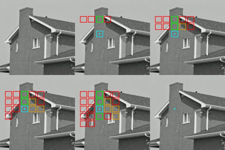
 It is important to remember that each pixel belong to $W\times W$ patches. So, after having
denoised each patch in the image we have as many pixel estimates. One can benefit from
those various estimates by combining them rather than just selecting the value corresponding
to the central position (cf. animation). The first solution propsed was to combine with a
uniform averaging the pixels estimates. Though by considering weighted average with
weights proportionnal to the inverse of the estimated variance, one can reduce the common
"halo of noise" created by the NLM around the edges.
Various Reprojections (Box-kernel)
|
Central PSNR=28.19 |
Uniform Average PSNR=28.68 |
Weighted Average PSNR=29.13 |
 |
 |
 |
Papers:
"From Patches to Pixels in Non-Local methods: Weighted-Average Reprojection"
J. Salmon and Y. Strozecki, ICIP, 2010, PDF. "Patch Reprojections for Non Local Methods"
J. Salmon and Y. Strozecki, Signal Processing, vol.92, pp. 477 - 489, 2012. PDF.
Corresponding Matlab Demo and toolbox ZIP.
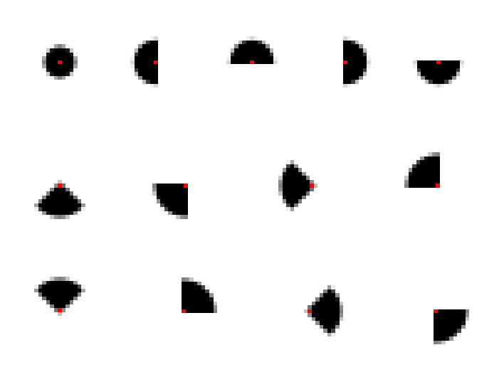
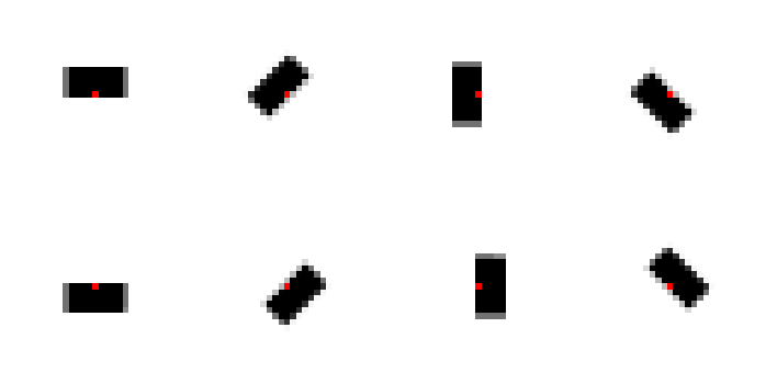
Another method consider to reduce the "halo of noise" due to the NLM, is to generalize the shape of the patches. Instead of using simple square patches, we propose to extend the NLM algorithm with more general families of shapes. Examples are classical squares, disks, but also bands and pie (cf. figure). The main point of this work is define a pertinent tool to locally aggregate the various estimations obtained for each pixel thanks to each shape. The technical tool we consider is the SURE (Stein Unbaised Risk Estimate), based on the Stein's Lemma. We apply the SURE to the NLM using shapes, instead of using SURE to simply determine the bandwith or the patch width.
\begin{equation}\newcommand{\ihat}{\hat{\itrue}} \ihat(\boldx)= \frac{\sum_{\boldx' \in \Omega} \wnlm{\boldx}{\boldx'} \inoisy(\boldx')}{\sum_{\boldx' \in \Omega} \wnlm{\boldx}{\boldx'}} \, , \end{equation} where the weights $\wnlm{\boldx}{\boldx'}$ depend on patches around $\boldx$ and $\boldx'$. The denominator is a normalizing factor which ensures the weights sum to one. The original weights in the NL-Means are of the following form: \begin{equation}\label{eq:nlm_weights} \wnlm{\boldx}{\boldx'}= \varphi \left( \frac{\|\patch_{\boldx} -\patch_{\boldx'}\|_{2,a}^2}{2h^2} \right) \, , \end{equation} where $h>0$ is the bandwidth parameter, $\varphi$ is the kernel used to measure similarity between patches, $\|\cdot\|_{2,a}$ is a weighted Euclidean norm using a Gaussian kernel, and $a$ is the bandwidth that controls the concentration of the kernel around the central pixel. In order to deal with patches of arbitrary shapes, we reformulate the way the distance between two pixels is measured in terms of patches. The weighted Euclidean distance $\|\cdot\|_{2,a}$ used above can be generalized using the following expression: \begin{equation}\label{eq:shape_distance} d^2_{\mathbf S}(\boldx,\boldx')=\sum_{\tau \in \Omega} \mathbf{S}(\tau) (\inoisy(\boldx+\tau)-\inoisy(\boldx'+\tau))^2 \, , \end{equation} where $\mathbf{S}$ encodes the shape we aim at.Squares: To begin with, we apply our framework to the most commonly used shapes, i.e., the square shapes of odd length (so the squares have centers we can consider). For instance, choosing: \begin{equation}\label{eq:lambda_simple_nlm} \mathbf{S}(\tau)=\left \{ \begin{array}{ll} 1, \, &\mbox{ if } \|\tau\|_\infty \le \frac{p-1}{2}\, ,\\ \\ 0, \, &\mbox{ otherwise}, \end{array} \right. \end{equation} leads to the classical (simplified) NL-Means definition with square patches of size $p \times p$ and distance between patches measured by the Euclidean norm.
Gaussian The original, but less common choice, is to set: \begin{equation}\label{eq:lambda_original_nlm} \mathbf{S}(\tau)=\left \{ \begin{array}{ll} \exp(-(\tau_1^2+\tau_2^2)/2a^2), \, &\mbox{ if } \|\tau\|_\infty \le \frac{p-1}{2}\, ,\\ \\ 0, \, &\mbox{ otherwise.} \end{array} \right. \end{equation} The last equation means that the norm $ \|\cdot\|_{2,a}$ is used to measure the distance between patches in the definition of the NL-Means. This limits the influence of square patches corners and leads to a more isotropic comparison between patches.
Disks: Disk shapes are defined in the same way, using the Euclidean norm instead:
\begin{equation}
\mathbf{S}(\tau)=\left \{ \begin{array}{ll}
1, \, &\mbox{ if } \|\tau\|_2 \le \frac{p-1}{2}\, ,\\
\\
0, \, &\mbox{ otherwise.}
\end{array} \right.
\end{equation}
 A non-binary version may also be defined for pixels crossed by the boundary.
Pie slices: We study a family of shapes, denoted as "pie", whose elements are defined with three parameters: two angles and a radius. These shapes represent a portion of a disk delimited byeq two lines and surrounding the discrete central pixel.
Bands: This family of shapes is simply composed of rectangles, potentially rotated and
decentered with respect to the pixel of interest.

We have also provided a fast implementation of the method thanks to FFT calculations. Moreover, we have considered several rules to aggregates thanks to SURE the shape-based estimates obtained.
| Example of using several shapes and combining them | The shapes used |
 |
 |
Papers:
"Anisotropic Non-Local Means with Spatially Adaptive Patch Shapes"
C.-A. Deledalle J. Salmon, V. Duval, SSVM 2011, PDF.
"Non-Local Methods with Shape-Adaptive Patches (NLM-SAP)"
C.-A. Deledalle J. Salmon, V. Duval, J. Math. Imaging Vis., vol.43, pp. 103-120, 2012, PDF.
Corresponding Matlab DEMO and toolbox ZIP.
